
SLIDE 1
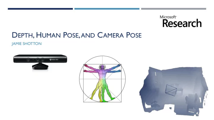
DEPTH, HUMAN POSE, AND CAMERA POSE
JAMIE SHOTTON
Recognises your face and voice Kinect Adventures What the Kinect - - PowerPoint PPT Presentation
D EPTH , H UMAN P OSE , AND C AMERA P OSE JAMIE SHOTTON Depth sensing camera Tracks 20 body joints in real time Recognises your face and voice Kinect Adventures What the Kinect Sees top view side view depth image (camera view)
JAMIE SHOTTON
Kinect Adventures
top view side view depth image (camera view)
What the Kinect Sees
Structured light
x y z
baseline imaging plane
depth d1
depth d2
Depth Makes Vision That Little Bit Easier
Only works well lit Background clutter Scale unknown Color and texture variation
Works in low light Background removal easier Calibrated depth readings Uniform texture
Joint work with Shahram Izadi, Richard Newcombe, David Kim, Otmar Hilliges, David Molyneaux, Pushmeet Kohli, Steve Hodges, Andrew Davison, Andrew Fitzgibbon. SIGGRAPH, UIST and ISMAR 2011.
Camera drift
ROADMAP
THEVITRUVIAN MANIFOLD [CVPR 2012] SCENE COORDINATE REGRESSION [CVPR 2013]
Jonathan Taylor Jamie Shotton Toby Sharp Andrew Fitzgibbon CVPR 2012
Human Pose Estimation
In this work:
Given some image input, recover the 3D human pose:
Joint positions and angles
Why is Pose Estimation Hard?
A Few Approaches
Regress directly to pose?
e.g. [Gavrila ’00] [Agarwal & Triggs ’04]
Per-Pixel Body Part Classification
[Shotton et al. ‘11]
Per-Pixel Joint Offset Regression
[Girshick et al. ‘11]
Detect and assemble parts?
e.g. [Felzenszwalb & Huttenlocher ’00] [Ramanan & Forsyth ’03] [Sigal et al. ’04]
Detect parts?
e.g. [Bourdev & Malik ‘09] [Plagemann et al. ‘10] [Kalogerakis et al. ‘10]
body joint hypotheses
front view side view top view
input depth image body parts
BPC Clustering
Background: Learning Body Parts for Kinect
[Shotton et al. CVPR 2011]
Train invariance to: Record mocap
100,000s of poses
Retarget to varied body shapes Render (depth, body parts) pairs
[Vicon]
Depth Image Features
– very fast to compute
input depth image
x
Δ
x
Δ
x
Δ x Δ
x
Δ
x
Δ
f(x; v) = 𝑒 x − 𝑒(x + Δ)
depth image coordinate
feature response Background pixels d = large constant scales inversely with depth
Δ = 𝐰 𝑒 x
Decision tree classification
image window centred at x
no no yes yes
P(c) P(c)
f(x; v1) > θ1 f(x; v2) > θ2
no yes
P(c) P(c)
f(x; v3) > θ3
Training Decision Trees
Sn = x f(x; vn) > θn
no yes
c Pr(c)
body part c Pn(c)
c Pl(c)
Take (v, θ) that maximises information gain:
n l r
Goal: drive entropy at leaf nodes to zero
reduce entropy
[Breiman et al. 84]
for all pixels
Δ𝐹 = − 𝑇l 𝑇𝑜 𝐹(Sl) − 𝑇r 𝑇𝑜 𝐹(Sr)
Decision Forests Book
input depth inferred body parts
no tracking or smoothing
body joint hypotheses
front view side view top view
input depth image body parts
BPC Clustering
front view top view side view
input depth inferred body parts inferred joint position hypotheses
no tracking or smoothing
Single frame at a time –> robust Large training corpus -> invariant Fast, parallel implementation Skeleton does not explain the depth data Limited ability to cope with hard poses
Body Part Recognition in Kinect
Explain the data directly with a mesh model
[Ballan et al. ‘08] [Baak et al. ‘11]
Many local minima
Highly sensitive to initial guess
Potentially slow
A few approaches
𝑆l_arm(𝜄)
𝑚 𝜄
relating its local coordinate system to the world:
𝑆global(𝜄)
𝑈
root 𝜄 = 𝑆global(𝜄)
𝑈
𝑚 𝜄
= 𝑈parent 𝑚 𝜄 𝑆𝑚(𝜄)
Human Skeleton Model
Linear Blend Skinning
𝑁 𝑣; 𝜄 =
𝑙=1 𝐿
𝛽𝑙𝑈𝑚𝑙 𝜄 𝑈
𝑚𝑙 −1 𝜄0 𝑞
Each vertex 𝑣
𝐿
with weights 𝛽𝑙 𝑙=1
𝐿
In a new pose 𝜄, the skinned position 𝑣 of is: Mesh in base pose 𝜄0
position in limb lk’s coordinate system position in world coordinate system
min
𝜄
min
𝑣1…𝑣𝑜 𝑗
𝑒(𝑦𝑗, 𝑁 𝑣𝑗; 𝜄 )
Test Time Model Fitting
𝑦𝑗 = 𝑁 𝑣𝑗; 𝜄
What pose is the model in?
Observed 3D Point Predicted 3D Point
𝐷𝑝𝑠𝑠𝑓𝑡𝑞𝑝𝑜𝑒𝑗𝑜 𝑁𝑝𝑒𝑓𝑚 𝑄𝑝𝑗𝑜𝑢𝑡: 𝑣1, … 𝑣𝑜 𝑃𝑐𝑡𝑓𝑠𝑤𝑓𝑒 𝑄𝑝𝑗𝑜𝑢𝑡: 𝑦1, … , 𝑦𝑜 𝑦𝑗
Note: simplified energy - more details to come
Optimizing
min
𝜄
min
𝑣1…𝑣𝑜 𝑗
𝑒(𝑦𝑗, 𝑁 𝑣𝑗; 𝜄 )
One-Shot Pose Estimation: An Early Result
Can we achieve a good result without iterating between pose 𝜄 and correspondences 𝑣1, … 𝑣n?
ground truth correspondences test depth image convergence visualization
Texture is mapped across body shapes and poses
From Body Parts to Dense Correspondences
increasing number of parts classification regression The “Vitruvian Manifold” Body Parts
The “Vitruvian Manifold” Embedding in 3D
v = 1 v = -1 u = -1 u = 1 w = -1
[L. Da Vinci, 1487]
w = 1
Geodesic surface distances approximated by Euclidean distance
Overview
inferred dense correspondences test images
regression forest
…
energy function
model parameters 𝜄 final optimized poses
front right top
training images
Discriminative Model: Predicting Correspondences
input images inferred dense correspondences
regression forest
…
training images
Learning the Correspondences
𝑦𝑗
render characters mocap
mean shift mode detection Each pixel-correspondence pair descends to a leaf in the tree
Learning a Regression Model at the Leaf Nodes
Inferring Correspondences
infer correspondences 𝑉
min
𝜄 𝐹(𝜄, 𝑉)
Full Energy
𝐹 𝜄, 𝑉 = 𝜇vis𝐹vis 𝜄, 𝑉 + 𝜇prior𝐹prior 𝜄 + 𝜇int𝐹int 𝜄
Energy is robust to noisy correspondences
𝜍(𝑓)
𝑓 = 0 𝑑𝑡(𝜄0) 𝑑𝑢(𝜄0)
“Easy” Metric: Average Joint Accuracy
0% 10% 20% 30% 40% 50% 60% 70% 80% 90% 100% 0.05 0.1 0.15 0.2
Joints average accuracy (% joints within distance D) D: max allowed distance to GT (m)
Our algorithm Given GT u Optimal θ 𝜄 𝑉
Results on 5000 synthetic images
0% 10% 20% 30% 40% 50% 60% 70% 80% 90% 100% 0.05 0.1 0.15 0.2 0.25 0.3
Worst-case accuracy (% frames with all joints within dist. D) D: max allowed distance to GT (m)
Our algorithm Given GT u Optimal θ
Hard Metric: “Perfect” Frame Accuracy
𝜄 𝑉
Results on 5000 synthetic images
0.09m 0.11m 0.17m 0.21m 0.45m D:
Comparison
0% 10% 20% 30% 40% 50% 60% 70% 0.05 0.1 0.15 0.2 0.25 0.3
Worst case accuracy (% frames with all joints within dist. D) D: max allowed distance to GT (m)
Our algorithm [Shotton et al. '11] (top hypothesis) [Girshick et al. 11] (top hypothesis) [Shotton et al. '11] (best of top 5) [Girshick et al. '11] (best of top 5)
Require an oracle Achievable algorithms Results on 5000 synthetic images
Vitruvian Manifold
Each frame fit independently: no temporal information used
– 𝑜𝑟 correspondences per view – viewing matrix 𝑄
𝑟 to register the scene
– let data points 𝑦𝑗𝑙 be 2D image coordinates – let 𝑄
𝑟 include a projection to 2D
– minimize re-projection error
Generalization to Multiple 3D/2D Views
min
𝜄 𝑟=1 𝑅 𝑗 𝑜𝑟
𝑒(𝑦𝑗𝑟, 𝑄
𝑟𝑁 𝑣𝑗𝑟; 𝜄 )
0.1 0.2 0.3 0.4 0.5 0.6 0.7 0.8 0.9 1 0.02 0.04 0.06 0.08 0.1 0.12 0.14 0.16 0.18 0.2
Worst case accuracy (% frames with all joints within dist. D) D: max allowed distance to GT (m)
2 silhouette views 3 silhouette views 5 silhouette views 1 depth view 2 depth views 5 depth views
Silhouette Experiment
– train invariance to body shape, size, and pose
– fast, accurate – auto-initializes using correspondences
JAMIE SHOTTON BEN GLOCKER CHRISTOPHER ZACH SHAHRAM IZADI ANTONIO CRIMINISI ANDREW FITZGIBBON [CVPR 2013]
Know this Observe this Where is this?
6D camera pose, 𝐼 (camera to scene transformation) Single RGB-D frame A world scene
APPLICATIONS
Lost or kidnapped robots Improving KinectFusion Augmented reality
TYPICAL APPROACHES TO CAMERA LOCALIZATION
Tracking – alignment relative to previous frame
e.g. [Besl & MacKay ‘92]
Key point detection → local descriptors → matching → geometric verification
e.g. [Holzer et al. ‘12], [Winder & Brown ‘07], [Lepetit & Fua ‘06], [Irschara et al. ‘09]
Whole key-frame matching
e.g. [Klein & Murray 2008] [Gee & Mayol-Cuevas 2012]
Epitomic location recognition
[Ni et al. 2009]
approximate precise
PROBLEMS IN REAL WORLD CAMERA LOCALIZATION
The real world is less exciting than vision researchers might like
The real world is big
KEY IDEA: SCENE COORDINATE REGRESSION Scene coordinate XYZ RGB color space
KEY IDEA: SCENE COORDINATE REGRESSION
Let each pixel predict direct correspondence
to 3D point in scene coordinates:
A B C
Input RGB Input Depth Desired Correspondences
A B C
Scene coordinate XYZ RGB color space 3D model from KinectFusion (only used for visualization)
SCENE COORDINATE REGRESSION
Offline approach to relocalization
observe a scene train a regression forest revisit the scene
Aim for really precise localization
e.g. suitable for AR overlays from a single frame without an explicit 3D model p ℳ𝑚1 𝐪
[Bunny: Stanford]
SCENE COORDINATE REGRESSION (SCORE) FORESTS
RGB Depth
tree 1
p ℳ𝑚1 𝐪 p
tree T
ℳ𝑚𝑈 𝐪 Depth & RGB features SCoRe Forest
𝜀1 𝐸(𝐪) 𝜀2 𝐸(𝐪)
Leaf Predictions ℳ𝑚 ⊂ ℝ3
𝐪
Forest Predictions ℳ 𝐪 =
𝑢
ℳ𝑚𝑢(𝐪)
TRAINING A SCORE FOREST
RGB-D frames with known camera poses 𝐼 Generate 3D pixel labels automatically:
𝐧 = 𝐼𝐲
Training Data
RGB Depth 𝐲 Labels 𝐧
Learning (standard)
Greedily train tree Reduction in spatial variance objective: Regression, not classification Mean shift to summarize distribution
at leaf 𝑚 into small set ℳ𝒎 ⊂ ℝ3
ROBUST CAMERA POSE OPTIMIZATION
pixel index camera pose robust error function correspondences predicted by forest at pixel 𝑗
Energy Function Optimization
Preemptive RANSAC [Nistér ICCV 2003] With pose refinement [Chum et al. DAGM 2003]
efficient updates to means & covariances
used by Kabsch SVD Only a small subset of pixels used
INLYING FOREST PREDICTIONS
Ground truth Inferred
Test images Inliers for six hypotheses
𝐼1 𝐼2 𝐼3 𝐼4 𝐼5 𝐼6
Camera pose
PREEMPTIVE RANSAC OPTIMIZATION
THE 7SCENES DATASET
Heads Pumpkin RedKitchen Stairs Dataset available from authors
BASELINES FOR COMPARISON
ORB matching
[Rublee et al. ICCV 2011]
FAST detector Rotation aware BRIEF descriptor Hashing for matching
Geometric verification
RANSAC & perspective 3 point Final refinement given inliers
Sparse Key-Points (RGB only) Tiny-Image Key-Frames (RGB & Depth)
Downsample to 40x30 pixels Blur Normalized Euclidean distance Brute-force search Interpolation of 100 closest poses
[Klein & Murray ECCV 2008] [Gee & Mayol-Cuevas BMVC 2012]
QUANTITATIVE COMPARISON
Choice of different image features Proportion of test frames with < 0.05m translational error and < 5○ angular error Metric: Results:
QUALITATIVE COMPARISON
ground truth DA-RGB SCoRe forest sparse baseline closest training pose
QUALITATIVE COMPARISON
ground truth DA-RGB SCoRe forest sparse baseline closest training pose
TRACK VISUALIZATION VIDEOS
ground truth DA-RGB SCoRe forest RGB sparse baseline single frame at a time – no tracking
AR VISUALIZATION
RGB input + AR overlay depth input + AR overlay rendering of model from inferred pose
single frame at a time – no tracking
[Bunny: Stanford]
SIMPLE ROBUST TRACKING
Add a single extra hypothesis to optimization: the result from previous frame
Single frame
AR VISUALIZATION WITH TRACKING
RGB input + AR overlay depth input + AR overlay rendering of model from inferred pose
simple robust frame-to-frame tracking enabled
[Bunny: Stanford]
MODEL-BASED REFINEMENT
Model-based refinement
requires 3D model of scene run rigid ICP from our inferred pose between observed image and model
0% 20% 40% 60% 80% 100% Chess Fire Heads Office Pumpkin RedKitchen Stairs
Proportion of frames correct
Baseline: Tiny-Image Depth Baseline: Tiny-Image RGB Baseline: Tiny-Image RGB-D Baseline: Sparse RGB Ours: Depth Ours: DA-RGB Ours: DA-RGB + D
[Besl & McKay PAMI 1992]
AR VISUALIZATION WITH TRACKING AND REFINEMENT
RGB input + AR overlay depth input + AR overlay rendering of model from inferred pose
simple robust frame-to-frame tracking and ICP-based model refinement enabled
[Bunny: Stanford]
Fire Scene
SCoRe Forest (single frame at a time) SCoRe Forest + simple robust frame-to-frame tracking SCoRe Forest + simple robust frame-to-frame tracking + ICP refinement to 3D model RGB input + AR overlay depth input + AR overlay rendering of model from inferred pose
[Bunny: Stanford]
Pumpkin Scene
RGB input + AR overlay depth input + AR overlay rendering of model from inferred pose SCoRe Forest (single frame at a time) SCoRe Forest + simple robust frame-to-frame tracking SCoRe Forest + simple robust frame-to-frame tracking + ICP refinement to 3D model
[Bunny, Armadillo: Stanford]
SCENE RECOGNITION
Chess Fire Heads Office Pumpkin RedKitchen Stairs Chess 100.0% 0.0% 0.0% 0.0% 0.0% 0.0% 0.0% Fire 2.0% 98.0% 0.0% 0.0% 0.0% 0.0% 0.0% Heads 0.0% 0.0% 100.0% 0.0% 0.0% 0.0% 0.0% Office 0.0% 0.5% 4.0% 95.5% 0.0% 0.0% 0.0% Pumpkin 0.0% 0.0% 0.0% 0.0% 100.0% 0.0% 0.0% RedKitchen 2.8% 1.2% 3.6% 0.0% 0.0% 92.4% 0.0% Stairs 0.0% 0.0% 10.0% 0.0% 0.0% 0.0% 90.0%
Train one SCoRe Forest per scene Test frame against all scenes Scene with lowest energy wins Single frame only
SCENE COORDINATE REGRESSION - SUMMARY
Scene coordinate regression forests
provide a single-step alternative to detection/description/matching pipeline can be applied at any valid pixel, not just at interest points allow accurate relocalization without explicit 3D model
Tracking-by-detection is approaching temporal tracking accuracy
Unifying principal:
Per-pixel regression and per-image model fitting
Depth cameras are having huge impact Decision forests + big data
WRAP UP
Thank you!
With thanks to:
Andrew Fitzgibbon, Jon Taylor, Ross Girshick, Mat Cook, Andrew Blake, Toby Sharp, Pushmeet Kohli, Ollie Williams, Sebastian Nowozin, Antonio Criminisi, Mihai Budiu, Duncan Robertson, John Winn, Shahram Izadi The whole Kinect team, especially: Alex Kipman, Mark Finocchio, Ryan Geiss, Richard Moore, Robert Craig, Momin Al-Ghosien, Matt Bronder, Craig Peeper