Recap: Reasoning Over Time 0.3 Markov models 0.7 X 1 X 2 X 3 X 4 - - PowerPoint PPT Presentation

Recap: Reasoning Over Time

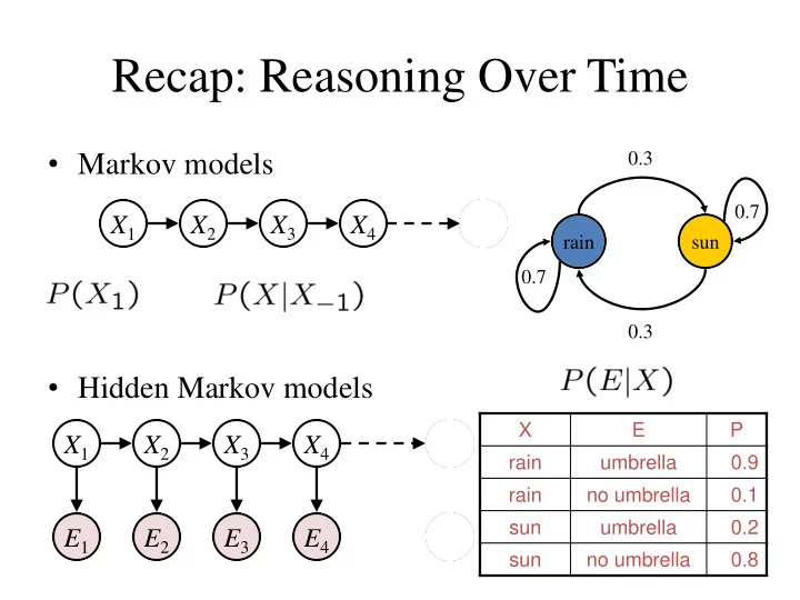
• Markov models
• Hidden Markov models

X2 X1 X3 X4

rain sun 0.7 0.7 0.3 0.3

X5 X2 E1 X1 X3 X4 E2 E3 E4 E5

X E P rain umbrella 0.9 rain no umbrella 0.1 sun umbrella 0.2 sun no umbrella 0.8

Passage of Time

• Assume we have current belief P(X | evidence to date)
• Then, after one time step passes:
• Or, compactly:
• Basic idea: beliefs get “pushed” through the transitions

– With the “B” notation, we have to be careful about what time step t the belief is about, and what evidence it includes

X2 X1

Example: Passage of Time

• As time passes, uncertainty “accumulates”

T = 1 T = 2 T = 5

Transition model: ghosts usually go clockwise

Example: Observation

• As we get observations, beliefs get reweighted,

uncertainty “decreases”

Before observation After observation

Example HMM

The Forward Algorithm

• We are given evidence at each time and want to know
• We can derive the following updates

We can normalize as we go if we want to have P(x|e) at each time step, or just once at the end…

Online Belief Updates

• Every time step, we start with current P(X | evidence)
• We update for time:
• We update for evidence:
• The forward algorithm does both at once (and doesn’t normalize)
• Problem: space is |X| and time is |X|2 per time step

X2 X1 X2 E2

• Voice Recognition:

http://www.youtube.com/watch?v=d9gDcHBmr3I

Filtering

• Elapse time: compute P( Xt | e1:t-1 )

Observe: compute P( Xt | e1:t ) X2 E1 X1 E2

<0.5, 0.5> Belief: <P(rain), P(sun)> <0.82, 0.18> <0.63, 0.37> <0.88, 0.12> Prior on X1 Observe Elapse time Observe

Particle Filtering

• Sometimes |X| is too big to use exact

inference

– |X| may be too big to even store B(X) – E.g. X is continuous – |X|2 may be too big to do updates

• Solution: approximate inference

– Track samples of X, not all values – Samples are called particles – Time per step is linear in the number of samples – But: number needed may be large – In memory: list of particles, not states

• This is how robot localization works

in practice

0.0 0.1 0.0 0.0 0.0 0.2 0.0 0.2 0.5

Representation: Particles

• Our representation of P(X) is now a

list of N particles (samples)

– Generally, N << |X| – Storing map from X to counts would defeat the point

• P(x) approximated by number of

particles with value x

– So, many x will have P(x) = 0! – More particles, more accuracy

• For now, all particles have a

weight of 1

14

Particles: (3,3) (2,3) (3,3) (3,2) (3,3) (3,2) (2,1) (3,3) (3,3) (2,1)

Particle Filtering: Elapse Time

• Each particle is moved by sampling its

next position from the transition model

– This is like prior sampling – samples’ frequencies reflect the transition probs – Here, most samples move clockwise, but some move in another direction or stay in place

• This captures the passage of time

– If we have enough samples, close to the exact values before and after (consistent)

Particle Filtering: Observe

• Slightly trickier:

– Don’t do rejection sampling (why not?) – We don’t sample the observation, we fix it – This is similar to likelihood weighting, so we downweight our samples based on the evidence – Note that, as before, the probabilities don’t sum to one, since most have been downweighted (in fact they sum to an approximation of P(e))

Particle Filtering: Resample

• Rather than tracking

weighted samples, we resample

• N times, we choose

from our weighted sample distribution (i.e. draw with replacement)

• This is analogous to

renormalizing the distribution

• Now the update is

complete for this time step, continue with the next one

Old Particles: (3,3) w=0.1 (2,1) w=0.9 (2,1) w=0.9 (3,1) w=0.4 (3,2) w=0.3 (2,2) w=0.4 (1,1) w=0.4 (3,1) w=0.4 (2,1) w=0.9 (3,2) w=0.3 New Particles: (2,1) w=1 (2,1) w=1 (2,1) w=1 (3,2) w=1 (2,2) w=1 (2,1) w=1 (1,1) w=1 (3,1) w=1 (2,1) w=1 (1,1) w=1

Robot Localization

• In robot localization:

– We know the map, but not the robot’s position – Observations may be vectors of range finder readings – State space and readings are typically continuous (works basically like a very fine grid) and so we cannot store B(X) – Particle filtering is often used

http://www.youtube.com/watch?v=kq JpuMNHF_g&feature=related http://www.youtube.com/watch? v=INLja6Ya3Ig&feature=related

Ghostbusters

• Plot: Pacman's grandfather, Grandpac,

learned to hunt ghosts for sport.

• He was blinded by his power, but could

hear the ghosts’ banging and clanging.

• Transition Model: All ghosts move

randomly, but are sometimes biased

• Emission Model: Pacman knows a “noisy”

distance to each ghost

1 3 5 7 9 11 13 15 Noisy distance prob True distance = 8