Recap: MDPs Markov decision processes: States S Start state s 0 - - PowerPoint PPT Presentation

Recap: MDPs

1

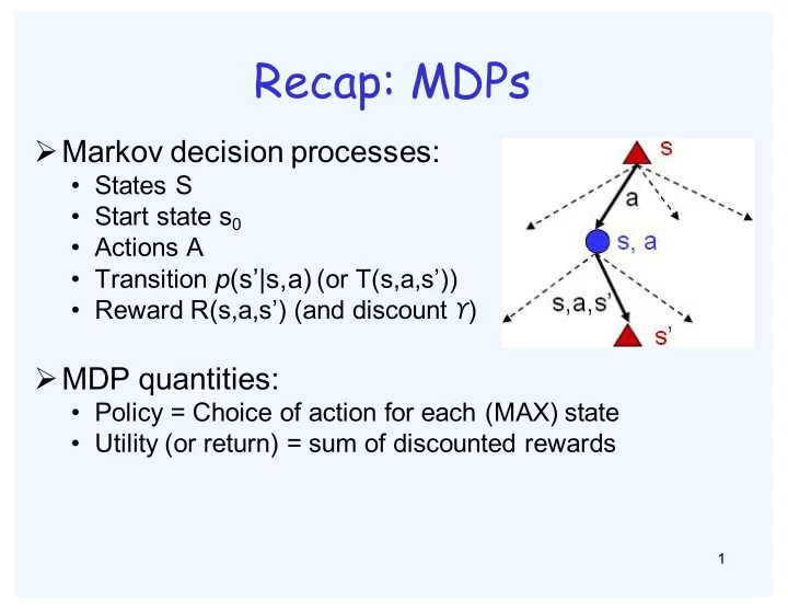
ØMarkov decision processes:

• States S
• Start state s0
• Actions A
• Transition p(s’|s,a) (or T(s,a,s’))
• Reward R(s,a,s’) (and discount ϒ)

ØMDP quantities:

• Policy = Choice of action for each (MAX) state
• Utility (or return) = sum of discounted rewards

Optimal Utilities

ØThe value of a state s:

• V*(s) = expected utility starting in s and

acting optimally

ØThe value of a Q-state (s,a):

• Q*(s,a) = expected utility starting in s,

taking action a and thereafter acting

• ptimally

ØThe optimal policy:

• π*(s) = optimal action from state s

Solving MDPs

3

ØValue iteration

• Start with V1(s) = 0
• Given Vi, calculate the values for all states for depth i+1:
• Repeat until converge
• Use Vi as evaluation function when computing Vi+1

ØPolicy iteration

• Step 1: policy evaluation: calculate utilities for some fixed

policy

• Step 2: policy improvement: update policy using one-step

look-ahead with resulting utilities as future values

• Repeat until policy converges

( ) ( ) ( ) ( )

1 '

max , , ' , , ' '

i i a s

V s T s a s R s a s V s γ

+

← + ⎡ ⎤ ⎣ ⎦

∑

ØDon’t know T and/or R, but can observe R

• Learn by doing
• can have multiple trials

4

Reinforcement learning

The Story So Far: MDPs and RL

5

Things we know how to do: ØIf we know the MDP

• Compute V*, Q*, π* exactly
• Evaluate a fixed policy π

ØIf we don’t know T and R

• If we can estimate the MDP then

solve

• We can estimate V for a fixed

policy π

• We can estimate Q*(s,a) for the
• ptimal policy while executing

an exploration policy

Techniques:

• Computation
• Value and policy

iteration

• Policy evaluation
• Model-based RL
• sampling
• Model-free RL:
• Q-learning

Model-Free Learning

6

ØModel-free (temporal difference) learning

• Experience world through trials

(s,a,r,s’,a’,r’,s’’,a’’,r’’,s’’’…)

• Update estimates each transition (s,a,r,s’)
• Over time, updates will mimic Bellman updates

( ) ( ) ( ) ( )

1 ' '

Q-Value Iteration (model-based, requires known MDP)

, , , ' , , ' max ', '

i i a s

Q s a T s a s R s a s Q s a γ

+

⎡ ⎤ ← + ⎣ ⎦

∑

( )

'

Q-Learning (model-free, requires only experienced transitions)

( , ) (1 ) ( , ) max ', '

a

Q s a Q s a r Q s a α α γ ⎡ ⎤ ← − + + ⎣ ⎦

Q-Learning

7

ØQ-learning produces tables of q-values:

Exploration / Exploitation

8

ØRandom actions (ε greedy)

• Every time step, flip a coin
• With probability ε, act randomly
• With probability 1-ε, act according to current

policy

Today: Q-Learning with state abstraction

9

ØIn realistic situations, we cannot possibly learn about every single state!

• Too many states to visit them all in training
• Too many states to hold the Q-tables in memory

ØInstead, we want to generalize:

• Learn about some small number of training states from

experience

• Generalize that experience to new, similar states
• This is a fundamental idea in machine learning, and we’ll

see it over and over again

Example: Pacman

10

ØLet’s say we discover through experience that this state is bad: ØIn naive Q-learning, we know nothing about this state or its Q-states: ØOr even this one!

Feature-Based Representations

11

ØSolution: describe a state using a vector of features (properties)

• Features are functions from states

to real numbers (often 0/1) that capture important properties of the state

• Example features:
• Distance to closest ghost
• Distance to closest dot
• Number of ghosts
• 1/ (dist to dot)2
• Is Pacman in a tunnel? (0/1)
• …etc
• Can also describe a Q-state (s,a)

with features (e.g. action moves closer to food)

Similar to a evaluation function

Linear Feature Functions

12

ØUsing a feature representation, we can write a Q function for any state using a few weights: ØAdvantage: more efficient learning from samples ØDisadvantage: states may share features but actually be very different in value!

Q s,a

( ) = w1 f1 s,a ( )+ w2 f2 s,a ( )++ wn fn s,a ( )

Function Approximation

13

ØQ-learning with linear Q-functions:

transition = (s,a,r,s’)

ØIntuitive interpretation:

• Adjust weights of active features
• E.g. if something unexpectedly bad happens, disprefer all

states with that state’s features

Q s,a

( ) = w1 f1 s,a ( )+ w2 f2 s,a ( )++ wn fn s,a ( )

( )

'

difference max ', ' ( , )

a

r Q s a Q s a γ ⎡ ⎤ = + − ⎣ ⎦

Q(s,a) ← Q(s,a)+α difference " # $ % wi ← wi +α difference " # $ % fi s,a

( )

Exact Q’s Approximate Q’s

Example: Q-Pacman

14

Q(s,a)= 4.0fDOT(s,a)-1.0fGST(s,a) fDOT(s,NORTH)=0.5 fGST(s,NORTH)=1.0 Q(s,a)=+1 R(s,a,s’)=-500 difference=-501 wDOT←4.0+α[-501]0.5 wGST ←-1.0+α[-501]1.0 Q(s,a)= 3.0fDOT(s,a)-3.0fGST(s,a)

a= North r = -500 s s’

Linear Regression

15

prediction y

 = w0 + w1 f1 x

( )

prediction y

 = w0 + w1 f1 x

( )+ w2 f2 x ( )

Ordinary Least Squares (OLS)

16

total error = yi − y



i

( )

2 i

∑

= yi − wk fk x

( )

k

∑

# $ % & ' (

2 i

∑

Minimizing Error

17

( ) ( ) ( ) ( ) ( ) ( ) ( )

2

1 error 2 error

k k k k k m k m m m k k m k

w y w f x w y w f x f x w w w y w f x f x α ⎛ ⎞ = − ⎜ ⎟ ⎝ ⎠ ∂ ⎛ ⎞ = − − ⎜ ⎟ ∂ ⎝ ⎠ ⎛ ⎞ ← + − ⎜ ⎟ ⎝ ⎠

∑ ∑ ∑

Imagine we had only one point x with features f(x): Approximate q update as a one-step gradient descent :

( )

max ( ', ') ( , )

m m a m

w r Q s Q f x a a w s α γ + − ⎡ ⎤ ← + ⎣ ⎦

“target” “prediction”

ØAs many as possible?

• computational burden
• overfitting

ØFeature selection is important

• requires domain expertise

18

How many features should we use?

Overfitting

19

ØMDPs

• Q1: value iteration
• Q2: find parameters that lead to certain optimal policy
• Q3: similar to Q2

ØQ-learning

• Q4: implement the Q-learning algorithm
• Q5: implement ε greedy action selection
• Q6: try the algorithm

ØApproximate Q-learning and state abstraction

• Q7: Pacman

ØTips

• make your implementation general

20

Overview of Project 3