Recall the Basics of Hypothesis Testing The level of significance , - - PowerPoint PPT Presentation

Recall the Basics of Hypothesis Testing

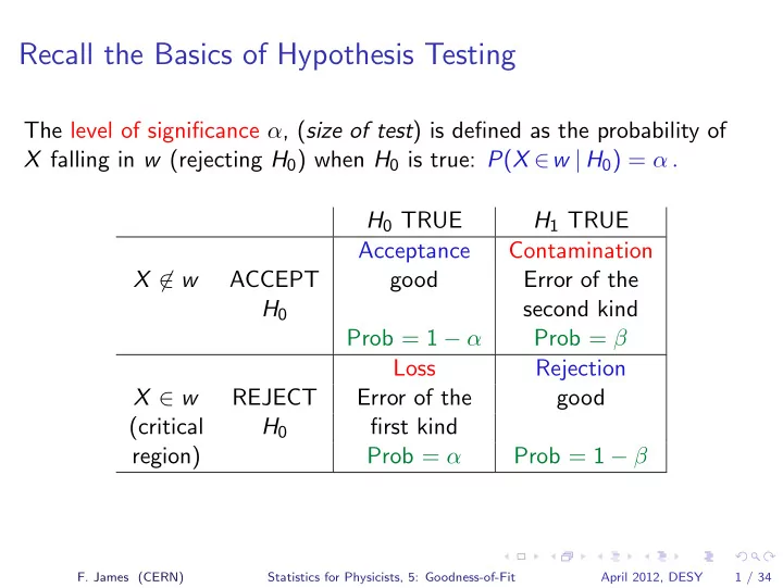
The level of significance α, (size of test) is defined as the probability of X falling in w (rejecting H0) when H0 is true: P(X ∈w | H0) = α . H0 TRUE H1 TRUE Acceptance Contamination X ∈ w ACCEPT good Error of the H0 second kind Prob = 1 − α Prob = β Loss Rejection X ∈ w REJECT Error of the good (critical H0 first kind region) Prob = α Prob = 1 − β

• F. James (CERN)

Statistics for Physicists, 5: Goodness-of-Fit April 2012, DESY 1 / 34

Goodness-of-Fit Testing

Goodness-of-Fit Testing (GOF)

As in hypothesis testing, we are again concerned with the test of a null hypothesis H0 with a test statistic T, in a critical region wα, at a significance level α. Unlike the previous situations, however, the alternative hypothesis, H1 is now the set of all possible alternatives to H0. Thus H1 cannot be formulated, the risk of second kind, β, is unknown, and the power of the test is undefined. Since it is in general impossible to know whether one test is more powerful than another, the theoretical basis for goodness-of-fit (GOF) testing is much less satisfactory than the basis for classical hypothesis testing. Nevertheless, GOF testing is quantitatively the most successful area of

• statistics. In particular, Pearson’s venerable Chi-square test is the most

heavily used method in all of statistics.

• F. James (CERN)

Statistics for Physicists, 5: Goodness-of-Fit April 2012, DESY 2 / 34

Goodness-of-Fit Testing GOF Testing: From the test statistic to the P-value.

GOF Testing: From the test statistic to the P-value.

Goodness-of-fit tests compare the experimental data with their p.d.f. under the null hypothesis H0, leading to the statement: If H0 were true and the experiment were repeated many times,

• ne would obtain data as far away (or further) from H0 as the
• bserved data with probability P.

The quantity P is then called the P-value of the test for this data set and

• hypothesis. A small value of P is taken as evidence against H0, which the

physicist calls a bad fit.

• F. James (CERN)

Statistics for Physicists, 5: Goodness-of-Fit April 2012, DESY 3 / 34

Goodness-of-Fit Testing GOF Testing: From the test statistic to the P-value.

From the test statistic to the P-value.

It is clear from the above that in order to construct a GOF test we need:

• 1. A test statistic, that is a function of the data and of H0, which is a

measure of the “distance” between the data and the hypothesis, and

• 2. A way to calculate the probability of exceeding the observed value of

the test statistic for H0. That is, a function to map the value of the test statistic into a P-value. If the data X are discrete and our test statistic is t = t(X) which takes on the value t0 = t(X0) for the data X0, the P-value would be given by: PX =

• X:t≥t0

P(X|H0) , where the sum is taken over all values of X for which t(X) ≥ t0.

• F. James (CERN)

Statistics for Physicists, 5: Goodness-of-Fit April 2012, DESY 4 / 34

Goodness-of-Fit Testing GOF Testing: From the test statistic to the P-value.

Example: Test of Poisson counting rate

Example of discrete counting data: We have recorded 12 counts in one year, and we wish to know if this is compatible with the theory which predicts µ = 17.3 counts per year. The obvious test statistic is the absolute difference |N − µ|, and assuming that the probability of n decays is given by the Poisson distribution, we can calculate the P-value by taking the sum in the previous slide. P12 =

• n:|n−µ|≥5.3

e−µµn n! =

12

• n=0

e−17.317.3n n! +

∞

• n=23

e−17.317.3n n! Evaluating the above P-value, we get P12 = 0.229. The interpretation is that the observation is not significantly different from the expected value, since one should observe a number of counts at least as far from the expected value about 23% of the time.

• F. James (CERN)

Statistics for Physicists, 5: Goodness-of-Fit April 2012, DESY 5 / 34

Goodness-of-Fit Testing GOF Testing: From the test statistic to the P-value.

Poisson Test Example seen visually

The length of the vertical bars is proportional to the Poisson probability of n (the x-axis) for H0 : µ = 17.3.

probability p 10 20 30 40 H0 nobs

• F. James (CERN)

Statistics for Physicists, 5: Goodness-of-Fit April 2012, DESY 6 / 34

Goodness-of-Fit Testing GOF Testing: From the test statistic to the P-value.

Distribution-free Tests

When the data are continuous, the sum becomes an integral: PX =

• X:t>t0

P(X|H0) , (1) and this can become quite complicated to compute, so that one tries to avoid using this form. Instead, one looks for a test statistic such that the distribution of t is known independently of H0. Such a test is called a distribution-free test. We consider here mainly distribution-free tests, such that the P-value does not depend on the details of the hypothesis H0, but only on the value of t, and possibly one

• r two integers such as the number of events, the number of bins in a

histogram, or the number of constraints in a fit. Then the mapping from t to P-value can be calculated once for all and published in tables, of which the well-known χ2 tables are an example.

• F. James (CERN)

Statistics for Physicists, 5: Goodness-of-Fit April 2012, DESY 7 / 34

Goodness-of-Fit Testing Pearson’s Chi-square Test

Pearson’s Chi-square Test

An obvious way to measure the distance between the data and the hypothesis H0 is to

• 1. Determine the expectation of the data under the hypothesis H0 .
• 2. Find a metric in the space of the data to measure the distance of the
• bserved data from its expectation under H0 .

When the data consists of measurements Y = Y1, Y2, . . . , Yk of quantities which, under H0 are equal to f = f1, f2, . . . , fk with covariance matrix ∼ V , the distance between the data and H0 is clearly: T = (Y − f)T ∼ V −1 (Y − f) This is just the Pearson test statistic usually called chi-square, because it is distributed as χ2(k) under H0 if the measurements Y are Gaussian-distributed. That means the P-value may be found from a table

• f χ2(k), or by calling PROB(T,k).
• F. James (CERN)

Statistics for Physicists, 5: Goodness-of-Fit April 2012, DESY 8 / 34

Goodness-of-Fit Testing Tests on Histograms

Pearson’s Chi-square test for histograms

Karl Pearson made use of the asymptotic Normality of a multinomial p.d.f. in order to find the (asymptotic) distribution of: T = (n − Np)T ∼ V −1 (n − Np) where ∼ V is the covariance matrix of the observations (bin contents) n and N is the total number of events in the histogram. In the usual case where the bins are independent, we have T = 1 N

k

• i=1

(ni − Npi)2 pi = 1 N

k

• i=1

n2

i

pi − N . This is the usual χ2 goodness-of-fit test for histograms. The distribution

• f T is generally accepted as close enough to χ2(k − 1) when all the

expected numbers of events per bin (Npi) are greater than 5. Cochran relaxes this restriction, claiming the approximation to be good if not more than 20% of the bins have expectations between 1 and 5.

• F. James (CERN)

Statistics for Physicists, 5: Goodness-of-Fit April 2012, DESY 9 / 34

Goodness-of-Fit Testing Tests on Histograms

Chi-square test with estimation of parameters

If the parent distribution depends on a vector of parameters θ = θ1, θ2, . . . , θr, to be estimated from the data, one does not expect the T statistic to behave as a χ2(k − 1), except in the limiting case where the r parameters do not actually affect the goodness of fit. In the more general and usual case, one can show that when r parameters are estimated from the same data, the cumulative distribution of T is intermediate between a χ2(k − 1) (which holds when θ is fixed) and a χ2(k − r − 1) (which holds for an optimal estimation method), always assuming the null hypothesis. The test is no longer distribution-free, but when k is large and r small, the two boundaries χ2(k − 1) and χ2(k − r − 1) become close enough to make the test practically distribution-free. In practice, the r parameters will be well chosen, and T will usually behave as χ2(k − r − 1) .

• F. James (CERN)

Statistics for Physicists, 5: Goodness-of-Fit April 2012, DESY 10 / 34

Goodness-of-Fit Testing Tests on Histograms

Binned Likelihood (Likelihood Chi-square)

Pearson’s Chi-square is a good test statistic when fitting a curve to points with Gaussian errors, but for fitting histograms, we can make use of the known distribution of events in a bin, which is not exactly Gaussian:

◮ It is Poisson-distributed if the bin contents are independent (no

constraint on the total number of events).

◮ Or it is Multinomial-distributed if the total number of events in the

histogram is fixed. reference: Baker and Cousins, Clarification of the Use of Chi-square and Likelihood Functions in Fits to Histograms NIM 221 (1984) 437 Our test statistic will be the binned likelihood, which Baker and Cousins called the likelihood chi-square because it behaves as a χ2, although it is derived as a likelihood ratio.

• F. James (CERN)

Statistics for Physicists, 5: Goodness-of-Fit April 2012, DESY 11 / 34

Goodness-of-Fit Testing Tests on Histograms

Binned Likelihood for Poisson bins

For bin contents ni that are Poisson-distributed with mean µi, we have: L =

• bins

e−µiµni

i /ni!

−2 ln L = 2

• i

[µi − ni ln µi + ln ni!] Now define L0 as L(ni = µi), the likelihood for a perfect fit: −2 ln L0 = 2

• i

[ni − ni ln ni + ln ni!] Now we subtract the last two equations above to get rid of the nasty term in n! and this gives the log of the likelihood ratio L/L0 : Poisson χ2

λ = −2 ln(L/L0) = 2

• i

[µi(θ) − ni + ni ln(ni/µi(θ))] where the last term is defined as =0 when ni = 0.

• F. James (CERN)

Statistics for Physicists, 5: Goodness-of-Fit April 2012, DESY 12 / 34

Goodness-of-Fit Testing Tests on Histograms

Binned Likelihood for Multinomial bins

For bin contents ni that are Multinomial-distributed with mean µi, we have: L = N!

• bins

(µi/N)ni/ni! −2 ln L = −2[ln N! − k ln N +

• i

(ni ln µi − ln ni!)] As before, we define L0 as L(ni = µi), the likelihood for a perfect fit, and taking the ratio L/L0 only one term remains, so we obtain: multinomial χ2

λ = −2 ln(L/L0) = 2

• i

[ni ln(ni/µi(θ))] where the terms in the sum are defined as =0 when ni = 0. Note that the multinomial form assumes that the µi obey the constraint

• i µi =

i ni = N , whereas with the Poisson form the fitted values of µi

will automatically satisfy this constraint.

• F. James (CERN)

Statistics for Physicists, 5: Goodness-of-Fit April 2012, DESY 13 / 34

Goodness-of-Fit Testing Tests on Histograms

Binned Likelihood as a GOF Test

Using the friendlier Poisson form, t = −2 ln λ = 2

• i

[µi(θ) − ni + ni ln(ni/µi(θ))] asymptotically obeys a Chi-square distribution, with number of degrees of freedom equal to the number of bins minus one. It is therefore a GOF test. Faced with the enormous popularity of Pearson’s T-statistic, binned likelihood is not used as much as it should be, so practical experience is somewhat limited, but all indications are that it is superior to Pearson’s T for histograms, both for parameter fitting and for GOF testing. If we make the bins more numerous and narrower, the efficiency as an estimator improves, but the power of the GOF test at some point degrades. In the limit of infinitely narrow bins, all ni are either zero or one, and the binned likelihood tends to the unbinned likelihood (not good for GOF).

• F. James (CERN)

Statistics for Physicists, 5: Goodness-of-Fit April 2012, DESY 14 / 34

Goodness-of-Fit Testing Other Tests on Binned Data

Runs test

A drawback of the T statistic is that the signs of the deviations (ni − Npi) are lost. The runs test is based on the signs of the deviations. The main interest of this test is that, for simple hypotheses, it is independent of the χ2 test on the same bins and thus brings in new information. Under hypothesis H0, all patterns of signs are equally probable. This simple fact allows us to write the following results [Wilks, p. 154]. Let M be the number of positive deviations, N the number of negative deviations, and R the total number of runs, where a run is a sequence of deviations of the same sign, preceded and followed by a deviation of opposite sign (unless at the end of the range of the variable studied). Then P(R = 2s) = 2 M−1

s−1

N−1

s−1

• M+N

M

• P(R = 2s − 1)

= M−1

s−2

N−1

s−1

• +

M−1

s−1

N−1

s−2

• M+N

M

• F. James (CERN)

Statistics for Physicists, 5: Goodness-of-Fit April 2012, DESY 15 / 34

Goodness-of-Fit Testing Other Tests on Binned Data

Runs test

The critical region is defined as improbably low values of R : R ≤ Rmin. Given the probability of R, one can compute Rmin corresponding to the significance level required. The expectation and variance of R are E(R) = 1 + 2MN M + N V (R) = 2MN(2MN − M − N) (M + N)2(M + N − 1) . Although the runs test is usually not as powerful as Pearson’s χ2 test, it is (asymptotically) independent of it and hence the two can be combined to produce an especially important test (see below, Combining Independent Tests).

• F. James (CERN)

Statistics for Physicists, 5: Goodness-of-Fit April 2012, DESY 16 / 34

Goodness-of-Fit Testing Tests without binning

Binned and Unbinned Data

Binned Data By combining events into histogram bins (called data classes in the statistical literature), some information is lost: the position of each event inside the bin. The loss of information may be negligible if the bin width is small compared with the experimental resolution, but in general one must expect tests on binned data to be inferior to tests on individual events. Tests on Unbinned Data Unfortunately, the requirement of distribution-free tests restricts the choice

• f tests for unbinned data, and we will consider only those based on the
• rder statistics (or empirical distribution function).

Since order statistics can be defined only in one dimension, this limits us to data depending on only one random variable, and to simple hypotheses H0 (no free parameters θ).

• F. James (CERN)

Statistics for Physicists, 5: Goodness-of-Fit April 2012, DESY 17 / 34

Goodness-of-Fit Testing Tests without binning

Order statistics

Given N independent observations X1, . . . , XN of the random variable X, let us reorder the observations in ascending order, so that X(1) ≤ X(2) ≤, . . . , ≤ X(N) (this is always permissible since the

• bservations are independent).

The ordered observations X(i) are called the order statistics. Their cumulative distribution is called the empirical distribution function or EDF. SN(X) =    X < X(1) i/N for X(i) ≤ X < X(i+1), i = 1, . . . , N − 1 . 1 X(N) ≤ X Note that SN(X) always increases in steps of equal height, N−1.

• F. James (CERN)

Statistics for Physicists, 5: Goodness-of-Fit April 2012, DESY 18 / 34

Goodness-of-Fit Testing Tests without binning

Order statistics

SN(X) TN(X) 1 X Xm

Example

• f

two cumulative distribu- tions, SN(X) and TN(X) For these two data sets, the maximum distance SN − TN

• ccurs at X = Xm.

We shall consider dif- ferent norms on the difference SN(X) − F(X) as test statistics.

• F. James (CERN)

Statistics for Physicists, 5: Goodness-of-Fit April 2012, DESY 19 / 34

Goodness-of-Fit Testing Smirnov - Cram´ er - von Mises test

Smirnov - Cram´ er - von Mises test

Consider the statistic W 2 = ∞

−∞

[SN(X) − F(X)]2f (X)dX , where f (X) is the p.d.f. corresponding to the hypothesis H0, F(X) is the cumulative distribution, and SN(X) is defined as above, which gives W 2 = X1

−∞

F 2(X)dF(X) +

N−1

• i=1

Xi+1

Xi

i N − F(X) 2 dF(X) + ∞

XN

[1 − F(X)]2dF(X) = 1 N

• 1

12N +

N

• i=1
• F(Xi) − 2i − 1

2N 2 , using the properties F(−∞) ≡ 0, F(+∞) ≡ 1.

• F. James (CERN)

Statistics for Physicists, 5: Goodness-of-Fit April 2012, DESY 20 / 34

Goodness-of-Fit Testing Smirnov - Cram´ er - von Mises test

Smirnov - Cram´ er - von Mises test

The Smirnov-Cram´ er-von Mises test statistic W 2 has mean and variance E(W 2) = 1 N 1 F(1 − F)dF = 1 6N V (W 2) = E(W 4) − [E(W 2)]2 = 4N − 3 180N3 . Smirnov has calculated the critical values of NW 2 Test size α Critical value of NW 2 0.10 0.347 0.05 0.461 0.01 0.743 0.001 1.168 It has been shown that, to the accuracy of this table, the asymptotic limit is reached when N ≥ 3.

• F. James (CERN)

Statistics for Physicists, 5: Goodness-of-Fit April 2012, DESY 21 / 34

Goodness-of-Fit Testing Smirnov - Cram´ er - von Mises test

Smirnov - Cram´ er - von Mises test

When H0 is composite, W 2 is not in general distribution-free. When X is many-dimensional, the test also fails, unless the components are

• independent. However, one can form a test to compare two distributions,

F(X) and G(X). Let the number of observations be N and M, respectively, and let the hypothesis be H0: F(X) = G(X). Then the test statistic is W 2 = ∞

−∞

[SN(X) − SM(X)]2d NF(X) + MG(X) N + M

• .

Then the quantity MN M + N W 2 has the critical values shown in the table above.

• F. James (CERN)

Statistics for Physicists, 5: Goodness-of-Fit April 2012, DESY 22 / 34

Goodness-of-Fit Testing Kolmogorov test

Kolmogorov test

The test statistic is now the maximum deviation of the observed distribution SN(X) from the distribution F(X) expected under H0. This is defined either as DN = max |SN(X) − F(X)| for all X

• r as

D±

N = max {±[SN(X) − F(X)]}

for all X , when one is considering only one-sided tests. It can be shown that the limiting distribution of √ NDN is lim

N→∞ P(

√ NDN > z) = 2

∞

• r=1

(−1)r−1 exp(−2r2z2) and that of √ ND±

N is

lim

N→∞ P(

√ ND±

N > z) = exp(−2z2) .

• F. James (CERN)

Statistics for Physicists, 5: Goodness-of-Fit April 2012, DESY 23 / 34

Goodness-of-Fit Testing Kolmogorov test

Kolmogorov Test

Alternatively, the probability statement above can be restated as lim

N→∞ P[2N(D± N )2 ≤ 2z] = 1 − e−2z2 .

Thus 4N(D±

N )2 have a χ2(2) distribution.

The limiting distributions are considered valid for N ≈ 80. We give some critical values of √ NDN. Test size α Critical value of √ NDN 0.01 1.63 0.05 1.36 0.10 1.22 0.20 1.07

• F. James (CERN)

Statistics for Physicists, 5: Goodness-of-Fit April 2012, DESY 24 / 34

Goodness-of-Fit Testing Kolmogorov test

Two-Sample Kolmogorov Test

The equivalent statistic for comparing two distributions SN(X) and SM(X) is DMN = max |SN(X) − SM(X)| for all X

• r, for one-sided tests

D±

MN = max {±[SN(X) − SM(X)]}

for all X . Then

• MN/(M + N)DMN has the limiting distribution of

√ NDN and

• MN/(M + N)D±

MN have the limiting distribution of

√ ND±

N .

• F. James (CERN)

Statistics for Physicists, 5: Goodness-of-Fit April 2012, DESY 25 / 34

Goodness-of-Fit Testing Kolmogorov test

Kolmogorov Test

Finally, one may invert the probability statement about DN to set up a confidence belt for F(X). The statement P{DN = max |SN(X) − F(X)| > dα} = α defines dα as the α-point of DN. If follows that P{SN(X) − dα ≤ F(X) ≤ SN(X) + dα} = 1 − α . Therefore, setting up a belt ±dα about (SN(X), the probability that F(X) is entirely within the belt is 1 − α (similarly dα can be used to set up

• ne-sided bounds). One can thus compute the number of observations

necessary to obtain F(X) to any accuracy. Suppose for example that one wants F(X) to precision 0.05 with probability 0.99, then one needs N = (1.628/0.05)2 ∼ 1000 observations.

• F. James (CERN)

Statistics for Physicists, 5: Goodness-of-Fit April 2012, DESY 26 / 34

Goodness-of-Fit Testing More refined tests based on the EDF

Better tests using the EDF

Users of the Kolmogorov test will probably notice that the maximum difference DN or DMN almost always occurs near the middle of the range

• f X. And it is constrained to be zero at the two end points.

This has led Anderson and Darling to propose an improved test which gives more weight to the ends of the range. The Anderson–Darling test is an example of a definite improvement on the Kolmogorov test, but one which comes at the expense of losing the distribution-free property. This means that the P-value must be computed differently depending on whether one is testing for Normally distributed data or uniformly distributed data, for example. Tests of this kind are outside the scope of this course; the reader is referred to the book of D’Agostino.

• F. James (CERN)

Statistics for Physicists, 5: Goodness-of-Fit April 2012, DESY 27 / 34

Goodness-of-Fit Testing Use of the likelihood function

The likelihood function is not a good test statistic (1)

Suppose that the N observations X have p.d.f. f (X) and log-likelihood function λ =

N

• i=1

ln f (Xi) . One can, in principle, compute the expectation and the variance of λ, EX(λ) = N

• ln f (X) · f (X)dX ,

VX(λ) = N

• [ln f (X) − N−1EX(λ)]2f (X)dX ,

and even higher moments, if one feels that the Normality assumption is not good enough. We can therefore convert the value of λ into a P-value.

• F. James (CERN)

Statistics for Physicists, 5: Goodness-of-Fit April 2012, DESY 28 / 34

Goodness-of-Fit Testing Use of the likelihood function

The likelihood function is not a good test statistic (2)

Unfortunately, the value of the likelihood does not make a good GOF test

• statistic. This can be seen in different ways, but the first clue should come

when we judge whether the likelihood is a measure of the “distance” between the data and the hypothesis. At first glance, we might expect it to be a good measure, since we know the maximum of the likelihood gives the best estimates of parameters. But in m.l. estimation, we are using the likelihood for fixed data as a function of the parameters in the hypothesis, whereas in GOF testing we use the likelihood for a fixed hypothesis as a function of the data, which is very different.

• F. James (CERN)

Statistics for Physicists, 5: Goodness-of-Fit April 2012, DESY 29 / 34

Goodness-of-Fit Testing Use of the likelihood function

The likelihood function is not a good test statistic (3)

Suppose for example that the hypothesis under test H0 is the uniform distribution (which can always be arranged by a simple coordinate transformation). For this hypothesis, it is easily seen that the likelihood has no power at all as a GOF test statistic, since all data sets (with the same number of events) have exactly the same value of the likelihood function, no matter how well they fit the hypothesis of uniformity. More extensive studies show a variety of examples where the value of the likelihood function has no power as a GOF statistic and no examples where it can be recommended. Joel Heinrich (2001) has written a report on that: CDF memo 5639.

• F. James (CERN)

Statistics for Physicists, 5: Goodness-of-Fit April 2012, DESY 30 / 34

Goodness-of-Fit Testing Combining Independent Tests

Combining Independent Tests

It may happen that two or more different tests may be applied to the same data, or the same test applied to different sets of data, in such a way that although no one test is significant by itself, the combination of tests becomes significant. When using a combined test, one must of course know the properties of the individual tests involved, and in addition two new problems arise: (a) establishing that the individual tests are independent (b) finding the best test statistic for the combined test (c) finding the significance level of the combined test.

• F. James (CERN)

Statistics for Physicists, 5: Goodness-of-Fit April 2012, DESY 31 / 34

Goodness-of-Fit Testing Combining Independent Tests

Combining Independent Tests, continued

• 1. Different tests on the same data set

Of all the usual distribution-free tests, only the Pearson χ2 test and the runs test are (asymptotically) independent [Kendall, II, p. 442]. Intuitively this is clear, since Pearson’s test does not depend on the ordering of the bins or on the signs of the deviations in each bin, while this is the only information used in the runs test. In fact, Pearson’s test, although probably the most generally used test of fit, has been criticized for its lack

• f power precisely because it does not take account of this information.
• 2. The same test on different data sets

Different data sets, even from the same experiment, are in general independent, so the same test can be applied to all the data sets, and the tests will be independent.

• F. James (CERN)

Statistics for Physicists, 5: Goodness-of-Fit April 2012, DESY 32 / 34

Goodness-of-Fit Testing Significance level of the combined test

Test statistic for the combined test

Suppose that two independent tests yield individual p-values p1 and p2. The obvious test statistic for the combined test is t = p1p2. It turns out that if nothing more is known (only the two p-values) it is not possible to find the optimal test statistic, but t = p1p2 is a reasonable choice giving equal weight to the two component tests. more on this later It might be supposed that the p-value of the combined test would be p12 = p1p2, but it is easily seen that if p1 and p2 are both uniformly distributed between zero and one, then the product p1p2 would not be uniform on the same interval. It can be shown that, with the test statistic t = p1p2, the p-value is p12 = t[1 − ln(t)] which is larger than t.

• F. James (CERN)

Statistics for Physicists, 5: Goodness-of-Fit April 2012, DESY 33 / 34

Goodness-of-Fit Testing Significance level of the combined test

P-value of the combined test

A better way to combine tests can be seen by considering how to combine the results of two Chi-square tests. Suppose we have applied Pearson’s test to two independent data sets, with the results χ2

1(n1) → p1

and χ2

2(n2) → p2

Clearly the combined test consists of adding the two χ2 and finding the p-value of that sum for n1+n2 degrees of freedom. This suggests that the general way to combine tests with p-values p1 and p2 is to convert the two p-values to χ2 and add the values of χ2. But for how many degrees of freedom? That depends on the relative ”weight” of the two tests, which may not be specified, in which case the solution to the problem is not unique.

• F. James (CERN)

Statistics for Physicists, 5: Goodness-of-Fit April 2012, DESY 34 / 34