Reporting bullying A recent SurveyUSA poll conducted in FL asked - - PowerPoint PPT Presentation

U 5: I    L 2: C-  S 101

Nicole Dalzell June 9, 2015

HT for comparing proportions: p1 = p2

Reporting bullying

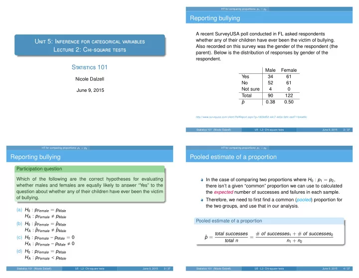
A recent SurveyUSA poll conducted in FL asked respondents whether any of their children have ever been the victim of bullying. Also recorded on this survey was the gender of the respondent (the parent). Below is the distribution of responses by gender of the respondent. Male Female Yes 34 61 No 52 61 Not sure 4 Total 90 122

ˆ

p 0.38 0.50

http://www.surveyusa.com/client/PollReport.aspx?g=1823ef50-44c7-4d2a-9efc-ead711b4ad9c Statistics 101 (Nicole Dalzell) U5 - L2: Chi-square tests June 9, 2015 2 / 37 HT for comparing proportions: p1 = p2

Reporting bullying

Participation question Which of the following are the correct hypotheses for evaluating whether males and females are equally likely to answer “Yes” to the question about whether any of their children have ever been the victim

• f bullying.

(a) H0 : pFemale = pMale HA : pFemale pMale (b) H0 : ˆ pFemale = ˆ pMale HA : ˆ pFemale ˆ pMale (c) H0 : pFemale − pMale = 0 HA : pFemale − pMale 0 (d) H0 : pFemale = pMale HA : pFemale < pMale

Statistics 101 (Nicole Dalzell) U5 - L2: Chi-square tests June 9, 2015 3 / 37 HT for comparing proportions: p1 = p2

Pooled estimate of a proportion

In the case of comparing two proportions where H0 : p1 = p2, there isn’t a given “common” proportion we can use to calculated the expected number of successes and failures in each sample. Therefore, we need to first find a common (pooled) proportion for the two groups, and use that in our analysis. Pooled estimate of a proportion

ˆ

p = total successes total n

= # of successes1 + # of successes2

n1 + n2

Statistics 101 (Nicole Dalzell) U5 - L2: Chi-square tests June 9, 2015 4 / 37

HT for comparing proportions: p1 = p2

Application exercise: Pooled proportion Calculate the estimated pooled proportion of males and females who said that one of their children has been a victim of bullying. Which sample proportion (ˆ pFemale or ˆ pMale) the pooled estimate is closer to? Why?

Male Female Yes 34 61 No 52 61 Not sure 4 Total 90 122 ˆ p 0.38 0.50

Statistics 101 (Nicole Dalzell) U5 - L2: Chi-square tests June 9, 2015 5 / 37 HT for comparing proportions: p1 = p2

Application exercise: HT for comparing proportions Conduct a hypothesis test, at 5% significance level, to determine if males and females are equally likely to answer “Yes” to the question about whether any of their children have ever been the victim of bully- ing.

Male Female Yes 34 61 No 52 61 Not sure 4 Total 90 122 ˆ p 0.38 0.50

Statistics 101 (Nicole Dalzell) U5 - L2: Chi-square tests June 9, 2015 6 / 37 HT for comparing proportions: p1 = p2 Statistics 101 (Nicole Dalzell) U5 - L2: Chi-square tests June 9, 2015 7 / 37 Recap

Recap - inference for one proportion

Population parameter: p, point estimate: ˆ p Conditions:

independence

• random sample and 10% condition

at least 10 successes and failures

• if not → randomization

Standard error: SE =

• p(1−p)

n

for CI: use ˆ p for HT: use p0

Statistics 101 (Nicole Dalzell) U5 - L2: Chi-square tests June 9, 2015 8 / 37

Recap

Recap - comparing two proportions

Population parameter: (p1 − p2), point estimate: (ˆ p1 − ˆ p2) Conditions:

independence within groups

• random sample and 10% condition met for both groups

independence between groups at least 10 successes and failures in each group

• if not → randomization

SE(ˆ

p1−ˆ p2) =

• p1(1−p1)

n1

+ p2(1−p2)

n2

for CI: use ˆ p1 and ˆ p2 for HT:

when H0 : p1 = p2: use ˆ ppool = # suc1+#suc2

n1+n2

when H0 : p1 − p2 = (some value other than 0): use ˆ p1 and ˆ p2

• this is pretty rare

Statistics 101 (Nicole Dalzell) U5 - L2: Chi-square tests June 9, 2015 9 / 37 Recap

Reference - standard error calculations

• ne sample

two samples mean SE =

s √n

SE =

• s2

1

n1 + s2

2

n2

proportion SE =

• p(1−p)

n

SE =

• p1(1−p1)

n1

+ p2(1−p2)

n2

When working with means, it’s very rare that σ is known, so we usually use s. When working with proportions,

if doing a hypothesis test, p comes from the null hypothesis if constructing a confidence interval, use ˆ p instead

Statistics 101 (Nicole Dalzell) U5 - L2: Chi-square tests June 9, 2015 10 / 37 Chi square test of GOF

Categorical Data

We have been working with proportions and differences in proportions. What do we do if our categorical variable has more than two levels? Let’s see an example.

Statistics 101 (Nicole Dalzell) U5 - L2: Chi-square tests June 9, 2015 11 / 37 Chi square test of GOF Jury selection – random or not?

Jury selection

In a county where jury selection is supposed to be random, a civil rights group sues the county, claiming racial disparities in jury selection. Ethnicities of the people in the county who are eligible for jury duty is as follows (based on census results):

Ethnicity White Black

• Nat. Amer.

Asian & PI Other % in pop. 80.29% 12.06% 0.79% 2.92% 3.94%

The previous year, 2500 people were selected for jury duty; their ethnicities were as follows:

Ethnicity White Black

• Nat. Amer

Asian & PI Other jurors selected 1920 347 19 84 130

The court retains you as an independent expert to assess the statistical evidence that there was discrimination. You propose to formulate the issue as an hypothesis test.

Statistics 101 (Nicole Dalzell) U5 - L2: Chi-square tests June 9, 2015 12 / 37

Chi square test of GOF Jury selection – random or not?

Setting the hypotheses

What should the hypotheses be?

Remember: H0 always says “there’s nothing going on”.

Statistics 101 (Nicole Dalzell) U5 - L2: Chi-square tests June 9, 2015 13 / 37 Chi square test of GOF Jury selection – random or not?

Evaluating the hypotheses

As we are used to doing, we take a look at what the universe looks like under the null hypothesis. In this universe in which “the observed counts of jurors from various race/ethnicities follow the same ethnicity distribution in the population”, what do we expect our observed counts to be? To evaluate these hypotheses, we quantify how different the

• bserved counts are from the expected counts.

In other words, how different is our observed counts from what we should be seeing if the null hypothesis were true? Large deviations from what would be expected based on sampling variation (chance) alone provide strong evidence for the alternative hypothesis. This is called a goodness of fit test since we’re evaluating how well the observed data fit the expected distribution.

Statistics 101 (Nicole Dalzell) U5 - L2: Chi-square tests June 9, 2015 14 / 37 Chi square test of GOF Jury selection – random or not?

Application exercise: Expected counts in one-way tables Calculate expected number of jurors from each ethnicity if in fact the jury selection is random. n = 2500

Ethnicity White Black

• Nat. Amer.

Asian & PI Other % in pop. 80.29% 12.06% 0.79% 2.92% 3.94% Observed Counts 1920 347 19 84 130

Statistics 101 (Nicole Dalzell) U5 - L2: Chi-square tests June 9, 2015 15 / 37 Chi square test of GOF The chi-square test statistic

Anatomy of a test statistic

The general form of a test statistic is point estimate − null value SE of point estimate This construction is based on

1

identifying the difference between a point estimate and an expected value if the null hypothesis was true, and

2

standardizing that difference using the standard error of the point estimate.

These two ideas will help in the construction of an appropriate test statistic for count data.

Statistics 101 (Nicole Dalzell) U5 - L2: Chi-square tests June 9, 2015 16 / 37

Chi square test of GOF The chi-square test statistic

Chi-square statistic

When dealing with counts and investigating how far the observed counts are from the expected counts, we use a new test statistic called the chi-square (χ2) statistic.

χ2 statistic χ2 =

k

• i=1

(O − E)2

E where k = total number of cells

Statistics 101 (Nicole Dalzell) U5 - L2: Chi-square tests June 9, 2015 17 / 37 Chi square test of GOF The chi-square test statistic

Why square?

Squaring the difference between the observed and the expected

• utcome does two things:

Any standardized difference that is squared will now be positive. Differences that already looked unusual will become much larger after being squared. When have we seen this before?

Statistics 101 (Nicole Dalzell) U5 - L2: Chi-square tests June 9, 2015 18 / 37 Chi square test of GOF The chi-square distribution and finding p-values

The chi-square distribution

In order to determine if the χ2 statistic we calculated is considered unusually high or not we need to first describe its distribution. The chi-square distribution has just one parameter called degrees of freedom (df), which influences the shape, center, and spread of the distribution. When conducting a goodness of fit test to evaluate how well the

• bserved data follow an expected distribution, the degrees of

freedom are calculated as the number of cells (k) minus 1. df = k − 1

Remember: So far we’ve seen three other continuous distributions:

• normal distribution: unimodal and symmetric with two parameters: mean and standard

deviation

• T distribution: unimodal and symmetric with one parameter: degrees of freedom
• F distribution: unimodal and right skewed with two parameters: degrees of freedom or

numerator (between group variance) and denominator (within group variance)

Statistics 101 (Nicole Dalzell) U5 - L2: Chi-square tests June 9, 2015 19 / 37 Chi square test of GOF The chi-square distribution and finding p-values

Conditions for the chi-square test

1

Independence: Each case that contributes a count to the table must be independent of all the other cases in the table.

2

Sample size: Each particular scenario (i.e. cell) must have at least 5 expected cases. Failing to check conditions may unintentionally affect the test’s error rates.

Statistics 101 (Nicole Dalzell) U5 - L2: Chi-square tests June 9, 2015 20 / 37

Chi square test of GOF The chi-square distribution and finding p-values

p-value for a chi-square test

The p-value for a chi-square test is defined as the tail area above the calculated test statistic. This is because the test statistic is always positive, and a higher test statistic means a higher deviation from the null hypothesis.

p−value

Statistics 101 (Nicole Dalzell) U5 - L2: Chi-square tests June 9, 2015 21 / 37 Chi square test of GOF The chi-square distribution and finding p-values

Tail areas under the chi-square curve – manual

p-value = tail area under the chi-square distribution (as usual) For this we can use technology, or a chi-square probability table. This table works a lot like the t table, but only provides upper tail values.

5 10 15 20 25

Upper tail 0.3 0.2 0.1 0.05 0.02 0.01 0.005 0.001 df 1 1.07 1.64 2.71 3.84 5.41 6.63 7.88 10.83 2 2.41 3.22 4.61 5.99 7.82 9.21 10.60 13.82 3 3.66 4.64 6.25 7.81 9.84 11.34 12.84 16.27 4 4.88 5.99 7.78 9.49 11.67 13.28 14.86 18.47 5 6.06 7.29 9.24 11.07 13.39 15.09 16.75 20.52 6 7.23 8.56 10.64 12.59 15.03 16.81 18.55 22.46 7 8.38 9.80 12.02 14.07 16.62 18.48 20.28 24.32 · · ·

Statistics 101 (Nicole Dalzell) U5 - L2: Chi-square tests June 9, 2015 22 / 37 Chi square test of GOF The chi-square distribution and finding p-values

Tail areas under the chi-square curve – computation

While probability tables are very helpful in understanding how probability distributions work, and provide quick reference when computational resources are not available, they are somewhat archaic. Using R:

> pchisq(5.99, df = 4, lower.tail = FALSE) 0.1998963

Using a web applet: http://www.socr.ucla.edu/htmls/SOCR Distributions.html

Statistics 101 (Nicole Dalzell) U5 - L2: Chi-square tests June 9, 2015 23 / 37 Chi square test of GOF The chi-square distribution and finding p-values

Application exercise: Chi-square test of GOF Evaluate the hypotheses at 5% significance level. Does the jury se- lection appear to be random? Can we conclude that there is racial discrimination in jury selection?

Statistics 101 (Nicole Dalzell) U5 - L2: Chi-square tests June 9, 2015 24 / 37

Chi square test of GOF Example

Social Media Usage

Think about the population of the United States at large. What percent- age of individuals in each age bracket below do you think use social media?

Age 18-24 25-34 35-44 45-54 55-64 65+ % in pop.

Statistics 101 (Nicole Dalzell) U5 - L2: Chi-square tests June 9, 2015 25 / 37 Chi square test of GOF Example

Social Media

US eMarkerter conducted a survey and released the results in Jan- uary 2015. Here are the results for those that use social media in age brackets.

Age 18-24 25-34 35-44 45-54 55-64 65+ Observed( in millions) 28.3 35.3 29.7 26.4 19.7 14.6

http://www.statista.com/statistics/243582/us-social-media-user-age-groups/ Statistics 101 (Nicole Dalzell) U5 - L2: Chi-square tests June 9, 2015 26 / 37 Chi square test of GOF Example

Social Media

Application exercise: Do we have enough evidence to conclude that this data is different from what we predicted?

Age 18-24 25-34 35-44 45-54 55-64 65+ Observed( in millions) 28.3 35.3 29.7 26.4 19.7 14.6

http://www.statista.com/statistics/243582/us-social-media-user-age-groups/ Statistics 101 (Nicole Dalzell) U5 - L2: Chi-square tests June 9, 2015 27 / 37 Chi-square test of independence Obesity and marital status

Obesity and marital status

A study reported in the medical journal Obesity in 2009 analyzed data from the National Longitudinal Study of Adolescent Health. Obesity was defined as having a BMI of 30 or more. The research subjects were followed from adolescence to adulthood, and all the people in the sample were categorized in terms of whether they were obese and whether they were dating, cohabiting, or married. Does there appear to be a relationship between weight and relationship status? Dating Cohabiting Married Obese 81 103 147 Not Obese 359 326 277

Statistics 101 (Nicole Dalzell) U5 - L2: Chi-square tests June 9, 2015 28 / 37

Chi-square test of independence Obesity and marital status

Participation question If relationship status is the explanatory and weight status is the re- sponse variable, which of the following is the correct representation of the relationship? (a)

dating cohabiting married

• bese

not obese

(b)

• bese

not obese dating cohabiting married

Statistics 101 (Nicole Dalzell) U5 - L2: Chi-square tests June 9, 2015 29 / 37 Chi-square test of independence Obesity and marital status

Chi-square test of independence

The hypotheses are:

H0: Weight and relationship status are independent. Obesity rates do not vary by relationship status. HA: Weight and relationship status are dependent. Obesity rates do vary by relationship status.

The test statistic is calculated as

χ2

df = k

• i=1

(O − E)2

E where df = (R − 1) × (C − 1), where k is the number of cells, R is the number of rows, and C is the number of columns.

Note: We calculate df differently for one-way and two-way tables.

The p-value is the area under the χ2

df curve, above the calculated

test statistic.

Statistics 101 (Nicole Dalzell) U5 - L2: Chi-square tests June 9, 2015 30 / 37 Chi-square test of independence Expected counts in two-way tables

Application exercise: Expected counts in two-way tables What is the overall obesity rate in this sample? If in fact weight and relationship status are independent (i.e. if in fact H0 is true) how many

• f the dating people would we expect to be obese? How many of the

cohabiting and married?

Dating Cohabiting Married Obese 81 103 147 Not Obese 359 326 277

Statistics 101 (Nicole Dalzell) U5 - L2: Chi-square tests June 9, 2015 31 / 37 Chi-square test of independence Expected counts in two-way tables

Expected counts in two-way tables

Expected counts in two-way tables Expected Count = (row total) × (column total) table total

Statistics 101 (Nicole Dalzell) U5 - L2: Chi-square tests June 9, 2015 32 / 37

Chi-square test of independence Expected counts in two-way tables

Application exercise: Chi-square test of independence Test the hypothesis that relationship status and obesity are associated using a signify acne level of 0.05. Can we conclude from these data that living with someone jus making some people obese and that mar- rying jus making people even more obese? Can we conclude that

• besity affects relationship status?

Dating Cohabiting Married Obese 81 103 147 Not Obese 359 326 277

Statistics 101 (Nicole Dalzell) U5 - L2: Chi-square tests June 9, 2015 33 / 37 Chi-square test of independence Expected counts in two-way tables inference(weight,mar_stat,est="proportion", type = "ht", method = "theoretical", alternative = "greater") Response variable: categorical, Explanatory variable: categorical Chi-square test of independence Summary statistics: x y dating cohabiting married Sum

• bese

81 103 147 331 not obese 359 326 277 962 Sum 440 429 424 1293 H_0: Response and explanatory variable are independent. H_A: Response and explanatory variable are dependent. Check conditions: expected counts x y dating cohabiting married

• bese

112.64 109.82 108.54 not obese 327.36 319.18 315.46 Pearson’s Chi-squared test data: y_table X-squared = 30.8286, df = 2, p-value = 2.021e-07 Statistics 101 (Nicole Dalzell) U5 - L2: Chi-square tests June 9, 2015 34 / 37 Recap

Participation question Which of the following is false?

5 10 15 20 25 Degrees of Freedom 2 4 9

As the df increases, (a) the center of the χ2 distribution increases as well (b) the variability of the χ2 distribution increases as well (c) the shape of the χ2 distribution becomes more skewed (less like a normal)

Statistics 101 (Nicole Dalzell) U5 - L2: Chi-square tests June 9, 2015 35 / 37