Reading Recommended: ! Stollnitz, DeRose, and Salesin. Wavelets for - - PDF document

cse457-19-subdivision 1

Subdivision curves and surfaces

cse457-19-subdivision 2

Reading

Recommended: ! Stollnitz, DeRose, and Salesin. Wavelets for Computer Graphics: Theory and Applications, 1996, section 6.1-6.3, 10.2, A.5. Note: there is an error in Stollnitz, et al., section A.5. Equation A.3 should read: MV = VΛ

cse457-19-subdivision 3

Subdivision curves

Idea: ! repeatedly refine the control polygon ! curve is the limit of an infinite process

L → → →

3 2 1

P P P

i i

P Q

∞ →

= lim

cse457-19-subdivision 4

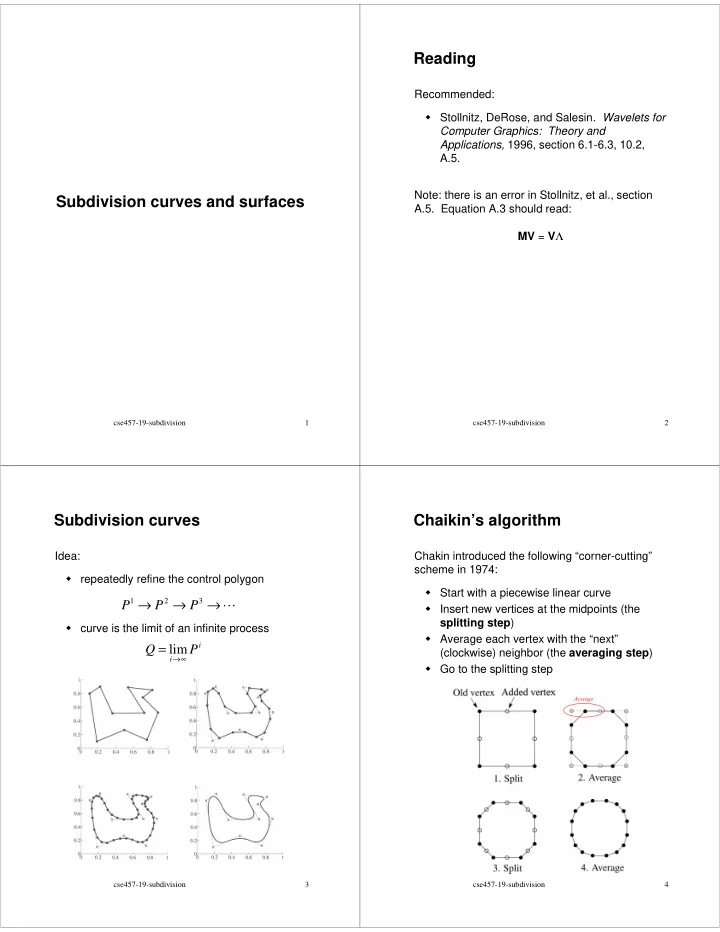
Chaikin’s algorithm

Chakin introduced the following “corner-cutting” scheme in 1974: ! Start with a piecewise linear curve ! Insert new vertices at the midpoints (the splitting step) ! Average each vertex with the “next” (clockwise) neighbor (the averaging step) ! Go to the splitting step

Average

cse457-19-subdivision 5

Averaging masks

The limit curve is a quadratic B-spline! Instead of averaging with the next neighbor, we can generalize by applying an averaging mask during the averaging step: In the case of Chaikin’s algorithm:

r =

−

= K K

1 1

( , , , , ) r r r r

cse457-19-subdivision 6

Lane-Riesenfeld algorithm (1980)

Use averaging masks from Pascal’s triangle: Gives B-splines of degree n+1. n=0: n=1: n=2:                           = n n n n r

n

, , 1 , 2 1 L

cse457-19-subdivision 7

Subdivide ad infinitum?

After each split-average step, we are closer to the limit curve. How many steps until we reach the final (limit) position? Can we push a vertex to its limit position without infinite subdivision? Yes!

Local subdivision matrix

Consider the cubic B-spline subdivision mask: Now consider what happens during splitting and averaging: We can write equations that relate points at one subdivision level to points at the previous:

( )

1 1 2 1 4

( ) ( ) ( ) ( ) ( ) ( ) ( ) ( ) ( ) ( )

1 * 1 * 1 1 * 0* 1 1 * 1 * 1 1 *

1 2 1 2 1 1 1 2 2 2 4 4 4 4 8 1 1 2 6 4 8 1 1 1 2 2 2 4 4 4 4 8

L L C R R C L L L L L C C C L R L R C C C R R R R R C C C

Q Q Q Q Q Q Q Q Q Q Q Q Q Q Q Q Q Q Q Q Q Q Q Q Q Q Q Q Q = + = + = + + = + = + = + + = + + = + + = + = +

cse457-19-subdivision 9

Local subdivision matrix

We can write this as a recurrence relation in matrix form: Where the Q’s are (for convenience) row vectors and S is the local subdivision matrix. Expanding this relation we get and so the limit position for Q0 is

1 1 1 1

4 4 1 1 6 1 8 0 4 4

j j L L j j C C j j R R j j

Q Q Q Q Q Q S

− − − −

            =                       = Q Q

3 2 1

Q S SSSQ SSQ SQ Q

j j j j j

= = = = =

− − −

L lim Q S Q

j j ∞ → ∞ = cse457-19-subdivision 10

Recipe for subdivision curves

Each subdivision scheme has its own evaluation mask, determined by eigenanalysis of the subdivision and averaging rules. After subdividing and averaging a few times to get a fine enough mesh, we can push each vertex in the mesh to its limit position by applying the evaluation mask. For Lane-Riesenfeld cubic B-spline subdivision, the evaluation mask is: Now we can cook up a simple procedure for creating subdivision curves: ! Subdivide (split+average) the control polygon a few times. Use the averaging mask. ! Push the resulting points to the limit positions. Use the evaluation mask.

( )

1 1 4 1 6

cse457-19-subdivision 11

DLG interpolating scheme (1987)

Slight modification to subdivision algorithm: ! splitting step introduces midpoints ! averaging step only changes midpoints For DLG (Dyn-Levin-Gregory), the averaging mask is: Since we are only changing the midpoints, the points after the averaging step do not move. 1 ( 2,5,10,5, 2) 16 r = − −

cse457-19-subdivision 12

Building complex models

We can extend the idea of subdivision from curves to surfaces…

cse457-19-subdivision 13

Subdivision surfaces

Chaikin’s use of subdivision for curves inspired similar techniques for subdivision surfaces. Iteratively refine a control polyhedron (or control mesh) to produce the limit surface using splitting and averaging steps.

j j

M

∞ →

= lim σ

M

1

M

2

M

∞

M L L

cse457-19-subdivision 14

Triangular subdivision

There are a variety of ways to subdivide a poylgon mesh. A common choice for triangle meshes is 4:1 subdivision – each triangular face is split into four subfaces:

Loop's subdivision scheme

Once again we can use masks for the averaging step: where These values, due to Charles Loop, are carefully chosen to ensure smoothness – namely, tangent plane or normal continuity. Note: tangent plane continuity is also know as G1 continuity for surfaces. 32 )) / 2 cos( 2 3 ( 4 5 ) ( ) ( )) ( 1 ( ) (

2

n n n n n n π β β β α + − = − =

1

( ) ( )

n

n n n α α + + + ← + Q Q Q Q L

cse457-19-subdivision 16

Loop's evaluation and tangent masks

As with subdivision curves, we can split and average a number of times and then push the points to their limit positions. where How do we compute the normal? Why would we want to? ε τ π β cos

i

3n (n)= (n)= (2 i/n) (n)

1 1 1 1 2 2 1 1 1 2 2

( ) ( ) ( ) ( ) ( ) ( ) ( ) ( )

n n n n n n

n n n n n n n n n ε ε τ τ τ τ τ τ

∞ ∞ ∞ −

+ + + = + = + + + = + + + Q Q Q Q T Q Q Q T Q Q Q L L L

cse457-19-subdivision 17

Recipe for subdivision surfaces

As with subdivision curves, we can now describe a recipe for creating and rendering subdivision surfaces: ! Subdivide (split+average) the control polyhedron a few times to get a reasonably fine mesh. Use the averaging mask. ! Compute two tangent vectors using the tangent masks. ! Compute the normal from the tangent vectors. ! Push the points to their limit positions. Use the evaluation mask. ! Render!

cse457-19-subdivision 18

Catmull-Clark subdivision

4:1 subdivision of triangles is sometimes called a face scheme for subdivision, as each face begets more faces. An alternative face scheme starts with arbitrary polygon meshes and inserts vertices along edges and at face centroids: Catmull-Clark subdivision: Note: after the first subdivision, all polygons are quadilaterals in this scheme.

cse457-19-subdivision 19

Adding creases

In some cases, we want a particular feature such as a crease to be preserved. For subdivision surfaces, we can just modify the subdivision mask: This gives rise to G0 continuous surfaces (i.e., having positional but not tangent plane continuity)

cse457-19-subdivision 20

Creases

Here’s an example using Catmull-Clark surfaces (based on subdividing quadrilateral meshes):

cse457-19-subdivision 21

Summary

What to take home: ! The meanings of all the boldfaced terms. ! How to perform the splitting and averaging steps on subdivision curves. ! How to perform mesh splitting steps for subdivision surfaces, especially Loop. ! How to construct and render subdivision surfaces from their averaging masks, evaluation masks, and tangent masks.