1 Limitations of Polygonal Meshes Planar facets (& silhouettes) - - PDF document

1

Introduction to Curves Modelling

• Points

– Defined by 2D or 3D coordinates

• Lines

– Defined by a set of 2 points

• Polygons

– Defined by a sequence of lines – Defined by a list of ordered points

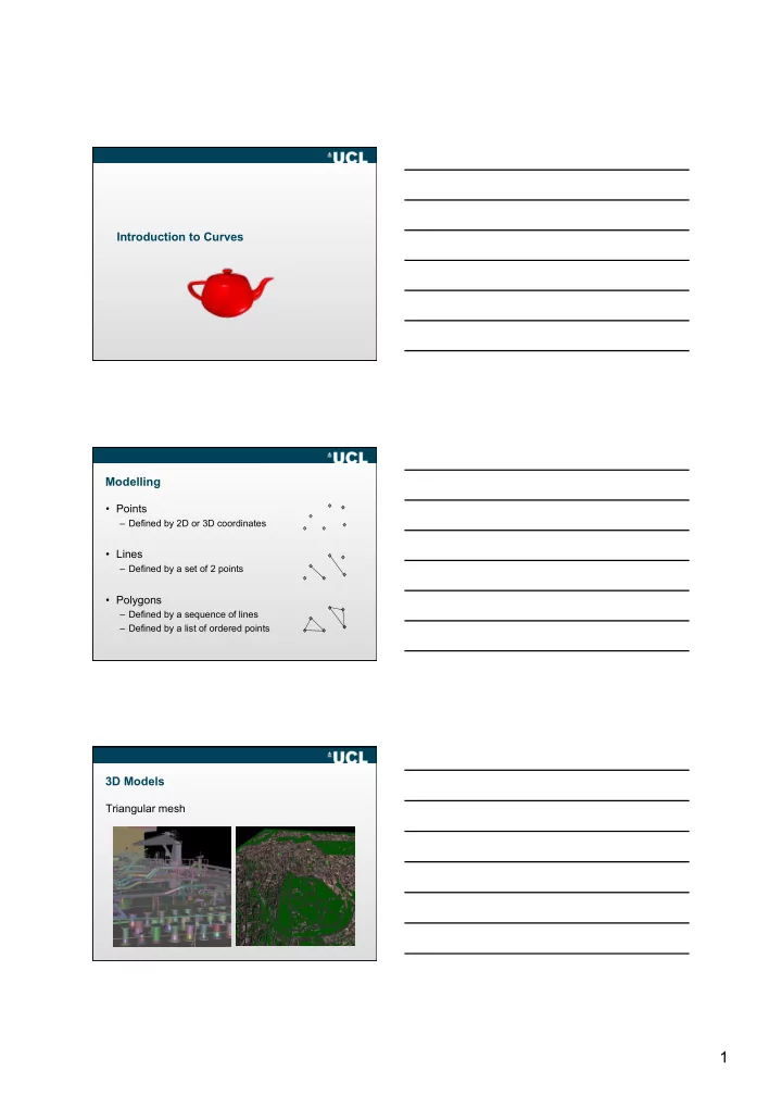
3D Models

Triangular mesh

2

Limitations of Polygonal Meshes

• Planar facets (& silhouettes)
• Fixed resolution
• Deformation is difficult
• No natural parameterization (for texture mapping)

Need to Disguise the Facets

• C0 continuous

– curve/surface has no breaks/gaps/holes

• G1 continuous

– tangent at joint has same direction

• C1 continuous

– curve/surface derivative is continuous – tangent at join has same direction and magnitude

• Cn continuous

– curve/surface through nth derivative is continuous – important for shading

Continuity Definitions

3

Let’s start with curves What if you want to have curves?

• Curves are often described with an analytic

equation

• It’s different from the discrete description of

polygons

• How do you deal with it in Computer Graphics?

First Solution

• Refine the number of points

– Can become extremely complex! – How do we interpolate?

• Draw freehand ---

– Too much data!

4

And for more complex curves?

Can I approximate this with line segments?

Interpolation

• How to interpolate between points?
• Which one corresponds to what we want?

Using curves for 3D modelling

• Modelled with curved surfaces, displayed with

polygons

5

Interpolation vs. Approximation Curves

Interpolation

curve must pass through control points

Approximation

curve is influenced by control points

Interpolation vs. Approximation Curves

• Interpolation curve – over constrained

→ lots of (undesirable?) oscillations

• Approximation curve – more reasonable?

Math background

• Polynomials

– n-th degree polynomial: p(t) = a0 + a1 t + a2 t2 + a3 t3 + … + an tn

• Affine map

– In one variable, defined as: f(t) = a + b t – A mapping is affine: f(α0*t0 + α1*t1) = α0*f(t0) + α1*f(t1) if α0 + α1

= 1

6

Interpolation

• On affine maps

– For t in [t1,t2] – Hence, for any affine f(): since t1 + t2 – t1 t2 – t t – t1 t = t2 – t1 t2 f(t1) + t2 – t1 t2 - t t - t1 f(t) = t2 – t1 f(t2) t2 – t1 t2 - t t - t1 t2 – t1 + = 1

Example of Affine Mapping

• Given and
• We can show:

Parameterised line segment

t between [0,1] P(t) = P0 (1-t) + t P1

P0 P1 P(t)

We can generalise to t in the range t1 to t2 (prev. slide) How to generalize to non-linear interpolation?

7

Symmetric Multi-Affine Maps

• 2-parameter version defined as:

– f(t1,t2) = c0 + c1 t1 +c2 t2 + c3 t1t2 (symmetry: c1=c2)

• Properties

– Affine separately on each of its arguments f(αa*t1a + αb*t1b, t2) = αa*f(t1a,t2) + αb*f(t1b,t2) f(t1,αa*t2a + αb*t2b) = αa*f(t1,t2a) + αb*f(t1,t2b) – Symmetry: Any permutation of the arguments results in the same value f(t1,t2) = f(t2,t1)

• Can be extended to more parameters!

Example

• Given
• Symmetry:
• Affine:

provided

Diagonalization of Symmetric Multi-Affine Maps

• Multi-Affine Map defined

– on hyper-cube [0,1]n, for n-variables

• In 2-parameter case:

– on square-domain [0,1]2

• Diagonalization: all arguments take same value

– F(t) := f(t,t) = c0 + (c1+c2) t + c3 t2

• New function F(t)

– Defined on diagonal of original domain

8

Blossoming theorem

• Strong connection between multi-affine maps and

polynomials

• Every n-argument multi-affine map has a

unique n-th degree polynomial as its diagonal

• Every n-th degree polynomial corresponds to a

unique symmetric n-argument multi-affine map, that has this polynomial as its diagonal

• The multi-affine map is called blossom (or polar

form)

Interpolation (through Diagonal)

• Recall interpolation on affine maps
• Consider t ∈ [r,s] in the 2-parameter case

f(r,s) + s – r s - t t - r f(t,s) = s – r f(s,s) f(t1) + t2 – t1 t2 - t t - t1 f(t) = t2 – t1 f(t2) f(r,r) + s – r s - t t - r f(r,t) = s – r f(r,s) f(r,t) + s – r s - t t - r f(t,t) = s – r f(s,t)

De Casteljau triangles

• Solution for f(t,t)

f(r,r) f(s,s) f(r,s) f(r,t) f(t,s) f(t,t)

9

Can be extend to degree n

• Solution for f(t,t,t)

f(r,r,r) f(r,s,s) f(r,r,s) f(r,r,t) f(r,t,s) f(r,t,t) f(s,s,s) f(t,s,s) f(t,t,t) f(s,t,t)

Bézier curves

• Use it to define Bézier curves:

f(t1,t2) = (x(t1,t2), y(t1,t2)) [= two f, one for each dim.]

• Given 3 points:

p0 = f(r,r) p1 = f(r,s) p2 = f(s,s)

• Interpolation by f(t,t) for any value of t.
• All points given by f(t,t) will lie on a curve

(2nd degree Bézier curve)

Three control points (quadratic Bézier)

• p0, p1, p2

p0 p1 p2 f(t,t) f(r,t) f(s,t) f(r,s) f(s,s) f(r,r)

t t t

10

Three control points (quadratic Bézier) With four control points (cubic Bézier)

• p0, p1, p2, p3

p0 p1 p2 p3 f(t,t,t) f(r,t,s) f(t,s,s) f(r,s,s) f(s,s,s) f(r,r,r) f(r,r,s) f(r,r,t) f(r,t,t) f(s,t,t)

t

With four control points (cubic Bézier)

11

Demo…

Properties for 3rd- degree Bézier curves

• End-points p0 = P(r) and p3 = P(s)
• Invariance of shape when change on the

parametric interval (affine transformation)

• The curve is bounded by the Convex hull given by

the control points

• An affine transformation of the control points is the

same as an affine transformation of any points of the curve

Properties for 3rd- degree Bézier curves

• If the control points are on a straight line, the

Bézier curve is a straight line

• The tangent vector of the curve at end points are

(for t=0 and t=1)

– P’(r) = 3(p1-p0) – P’(s) = 3(p3-p2)

12

Polynomial form of a Bézier curve

• Restriction to interval [0,1]
• 2nd degree

– f(0,t) = (1-t) f(0,0) + t f(0,1) = (1-t) P0 + t P1 – f(t,1) = (t-1) f(0,1) + t f(1,1) = (1-t) P1 + t P2 – F(t) = f(t,t) = (1-t) f(0,t) + t f(t,1) = (1-t)2 P0 + 2t(1-t) P1 + t2 P2 – Using the equation for interpolation

Polynomial form of a Bézier curve

• 3rd degree

– f(t,t,t) = (1-t)3 f(0,0,0) + 3t(1-t)2f(0,0,1) + 3(1-t)t2 f(0,1,1) + t3 f(1,1,1) = (1-t)3 P0 + 3t(1-t)2 P1 + 3(1-t)t2 P2 + t3 P3

Basis Functions

13

Other way of seeing a Bézier curve

• We drive the position on a curve using a

parameter u (for 2D or 3D): Q(u) = ( x(u), y(u) )

y x u=0 u=1

Four control points and [0,1]

• If we restrict t between [0,1], polynomial form:

– f(t,t,t) = (1-t)3 f(0,0,0) + 3t(1-t)2f(0,0,1) + 3(1-t)t2 f(0,1,1) + t3 f(1,1,1) = (1-t)3 P0 + 3t(1-t)2 P1 + 3(1-t)t2 P2 + t3 P3

• Which can be re-written in a more general case:

– Q(u) = ( x(u), y(u) ) = Σ Pi Bi(u) , where

Bi(u) = n i ui (1-u)n-i n i

=

n! i!(n-i)!

Bernstein basis

• B0(u) = (1-u)3
• B1(u) = 3 u (1-u)2
• B2(u) = 3 u2 (1-u)
• B3(u) = u3

Q(u) = U MB P = [u3 u2 u 1]

• 1 3 -3 1

3 -6 3 0

• 3 3 0 0

1 0 0 0 p0 p1 p2 p3

14

Bernstein basis

• Bi(u) are called Bernstein basis functions
• For 3rd degree:
• Property

– Any polynomial can be expressed uniquely as a linear combination of these basis functions

Bi(u) = n i ui (1-u)n-i

Higher-Order Bézier Curves

• > 4 control points
• Bernstein Polynomials as the basis functions
• Every control point affects the entire curve

– Not simply a local effect – More difficult to control for modeling

Tangent vectors

• For t in [0,1], consider

– F(t) = f(t,t,t) = (1-t)3 P0 + 3t(1-t)2 P1 + 3(1-t)t2 P2 + t3 P3 – F’(0) = 3 (P1-P0) – F’(1) = 3 (P3-P2)

• In general, for a Bézier curve of degree n:

– F’(0) = n (P1-P0) – F’(1) = n (Pn-Pn-1)

15

From polynomials, to blossoms, to control points

Problem

• F(t) = (X(t), Y(t)) = (1+3t2-t3, 1+3t-t3)
• Degree?
• Control points?
• F(t) = (x(t,t,t), y(t,t,t))

– x(t1,t2,t3) = ? – y(t1,t2,t3) = ? – P0 = ( , ) P1 = ( , ) P2 = ( , ) P3 = ( , )

Blossoming

• Easy, when paying attention to symmetry
• For our example:

– x(t,t,t) = 1+3t2-t3 → x(t1,t2,t3) = 1 + 3*(t0t1 + t1t2 + t0t2)/3 – t0*t1*t2 – y(t,t,t) = 1+3t-t3 → y(t1,t2,t3) = 1 + 3*(t0 + t1 + t2)/3 - t0*t1*t2

16

Deriving control points

• In general

– P0 = ( x(0,0,0), y(0,0,0) ) – P1 = ( x(0,0,1), y(0,0,1) ) – P2 = ( x(0,1,1), y(0,1,1) ) – P3 = ( x(1,1,1), y(1,1,1) )

• For our example

– P0 = (1,1) – P1 = (1,2) – P2 = (2,3) – P3

= (3,3)

Example

• How to derive 2nd-degree Bézier control points for

parabola: y=x2 ?

• Let’s try it!

Joining Bézier curves

• Better to join curves than raise the number of

controls points

– Avoid numerical instability – Local control of the overall shape C0 C1

17

Joining Bézier curves

• P0P1 defines a tangent to the curve at P0
• Tangent is common requirement to join two Bézier

curves together (with control points P0-3, Q0-3)

• This requires:

– The points P3 equals Q0 – Tangents to be equal

• I.e., P3 (=Q0), P2, Q1 are collinear

– Called C1 continuity (1st derivative is continuous) – C0: only positions are continuous (i.e. P3 = Q0)

Joining Bézier curves

P0 P1 P2 P3 Q0 Q1 Q2 Q3

Asymmetric: Curve goes through some control points but misses others

Conclusions

• It is possible to define and draw a curve with a

discrete representation

• All is needed are control points and interpolation

strategy

• We have scene Bézier curves

– From the DeCasteljau representation – From the Bernstein basis

18

Rational Bézier Curves

• Bézier curves cannot represent

many shapes

– E.g., no matter how high the degree a Bézier curve cannot represent a quadrant of a circle.

• Rational Bézier curves provide a

more powerful tool

• The example shows how a circle

can be exactly represented by the ratio of polynomials

• (Ex – find the corresponding

Bézier control points for numerator and denominator!)

Rational Bézier Curves

• To define a rational BC we

attach a ‘weight’ wi>0 to each control point.

• Note if all the weights are

equal then this is the same as a normal Bézier curve.

• The weights act as

‘atractors’ – the greater the weight the more the curve is pulled towards the corresponding point.

Conclusions

• Rational Bézier Curves more powerful!