Reading Further reading: Watt, sections 10.6 ,14.8 A. Glassner. - - PDF document

cse457-13-drt 1

Distribution Ray Tracing

cse457-13-drt 2

Reading

Further reading: Watt, sections 10.6 ,14.8

• A. Glassner. An Introduction to Ray Tracing.

Academic Press, 1989. [In the lab.] Robert L. Cook, Thomas Porter, Loren Carpenter. “Distributed Ray Tracing.” Computer Graphics (Proceedings of SIGGRAPH 84). 18 (3). pp. 137-145. 1984. James T. Kajiya. “The Rendering Equation.” Computer Graphics (Proceedings of SIGGRAPH 86). 20 (4). pp. 143-150. 1986.

cse457-13-drt 3

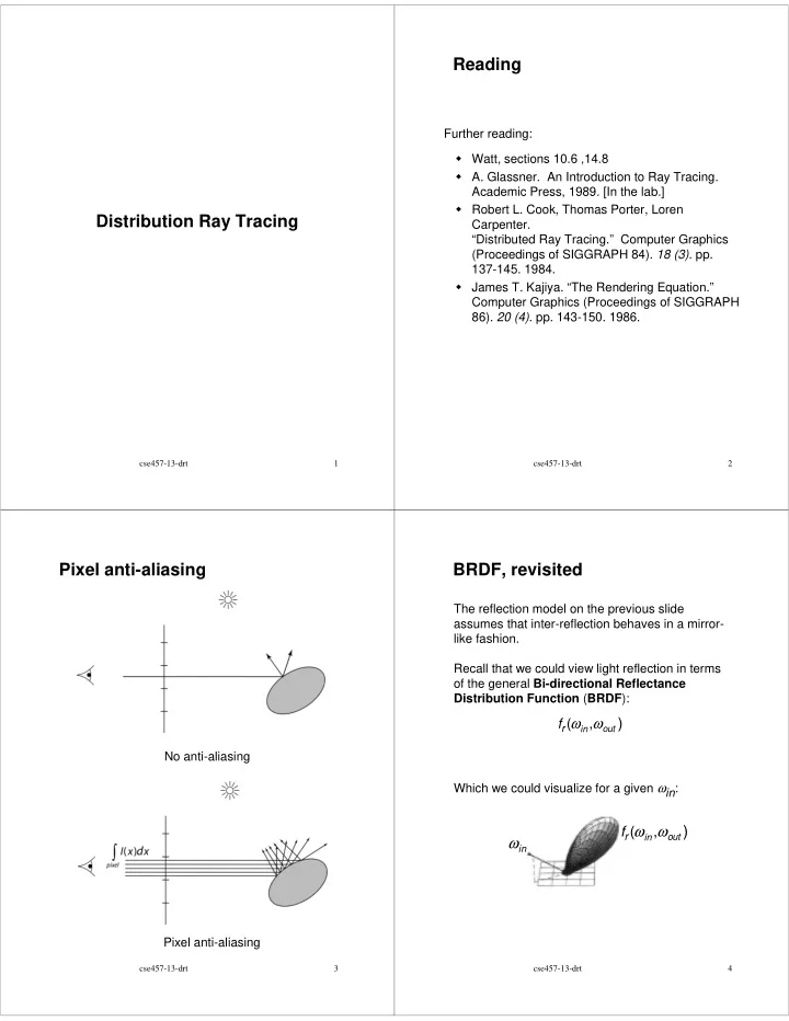
Pixel anti-aliasing

No anti-aliasing Pixel anti-aliasing

cse457-13-drt 4

BRDF, revisited

The reflection model on the previous slide assumes that inter-reflection behaves in a mirror- like fashion. Recall that we could view light reflection in terms

• f the general Bi-directional Reflectance

Distribution Function (BRDF): Which we could visualize for a given ωin:

( ,

)

• ut

in

r

f ω ω ( ,

)

• ut

in

r

f ω ω ωin

cse457-13-drt 5

Surface reflection equation

To compute the reflection from a real surface, we would actually need to solve the surface reflection equation: For a directional light with intensity L1 coming from direction direction, ω1, we can view the remaining directions as contributing zero, giving: We can plot the reflected light as a function of viewing angle for multiple light source contributions:

ω ω ω ω ω =∫ ( ) ( ) ( ,

)

H

• ut
• ut

in in in

r

I I f

d

ω ω ω =

1

1

( ) ( ,

)

• ut
• ut

r

I Lf

cse457-13-drt 6

Simulating gloss and translucency

The mirror-like form of reflection, when used to approximate glossy surfaces, introduces a kind of aliasing, because we are undersampling reflection (and refraction). For example: Distributing rays over reflection directions gives:

cse457-13-drt 7

Reflection anti-aliasing

Reflection anti-aliasing

cse457-13-drt 8

Full anti-aliasing

Full anti-aliasing…lots of nested integrals! Computing these integrals is prohibitively expensive, especially after following the rays recursively. We’ll look at ways to approximate high- dimensional integrals…

cse457-13-drt 9

Summing over ray paths

We can think of this problem in terms of enumerated rays: The intensity at a pixel is the sum over the primary rays: For a given primary ray, its intensity depends on secondary rays: Substituting back in:

1 ( )

n pixel i i

I I r n = ∑ = →

∑

( ) ( ) ( )

i ij r ij i j

I r I r f r r = →

∑∑

1 ( ) ( )

pixel ij r ij i i j

I I r f r r n

Summing over ray paths

We can incorporate tertiary rays next: Each triple i,j,k corresponds to a ray path: So, we can see that ray tracing is a way to approximate a complex, nested light transport integral with a summation over ray paths (of arbitrary length!). Problem: too expensive to sum over all paths. Solution: choose a small number of “good” paths.

= → →

∑∑∑

1 ( ) ( ) ( )

pixel ijk r ijk ij r ij i i j k

I I r f r r f r r n → →

ijk ij i

r r r

cse457-13-drt 11

Whitted integration

An anti-aliased Whitted ray tracer chooses very specific paths, i.e., paths starting on a regular sub- pixel grid with only perfect reflections (and refractions) that terminate at the light source. One problem with this approach is that it doesn’t account for non-mirror reflection at surfaces.

cse457-13-drt 12

Monte Carlo path tracing

Instead, we could choose paths starting from random sub-pixel locations with completely random decisions about reflection (and refraction). This approach is called Monte Carlo path tracing [Kajiya86]. The advantage of this approach is that the answer is known to be unbiased and will converge to the right answer.

cse457-13-drt 13

Importance sampling

The disadvantage of the completely random generation of rays is the fact that it samples unimportant paths and neglects important ones. This means that you need a lot of rays to converge to a good answer. The solution is to re-inject Whitted-like ideas: spawn rays to the light, and spawn rays that favor the specular direction.

cse457-13-drt 14

Stratified sampling

Another method that gives faster convergence is stratified sampling. E.g., for sub-pixel samples: We call this a jittered sampling pattern. One interesting side effect of these stochastic sampling patterns is that they actually injects noise into the solution (slightly grainier images). This noise tends to be less objectionable than aliasing artifacts.

cse457-13-drt 15

Distribution ray tracing

These ideas can be combined to give a particular method called distribution ray tracing [Cook84]: uses non-uniform (jittered) samples. replaces aliasing artifacts with noise. provides additional effects by distributing rays to sample:

• Reflections and refractions
• Light source area
• Camera lens area
• Time

[Originally called “distributed ray tracing,” but we will call it distribution ray tracing so as not to confuse with parallel computing.]

cse457-13-drt 16

DRT pseudocode

TraceImage() looks basically the same, except now each pixel records the average color of jittered sub- pixel rays. function traceImage (scene): for each pixel (i, j) in image do I(i, j) ← 0 for each sub-pixel id in (i,j) do s ← pixelToWorld(jitter(i, j, id)) p ← COP d ←(s - p).normalize() I(i, j) ← I(i, j) + traceRay(scene, p, d, id) end for I(i, j) I(i, j)/numSubPixels end for end function A typical choice is numSubPixels = 5*5.

cse457-13-drt 17

DRT pseudocode (cont’d)

Now consider traceRay(), modified to handle opaque glossy surfaces: function traceRay(scene, p, d, id): (q, N, material) ← intersect (scene, p, d) I ← shade(…) R ← jitteredReflectDirection(material, N, -d, id) I ← I + material.kr ∗ traceRay(scene, q, R, id) return I end function

cse457-13-drt 18

Pre-sampling glossy reflections

cse457-13-drt 19

Distributing rays over light source area gives:

Soft shadows

cse457-13-drt 20

The pinhole camera, revisited

Recall the pinhole camera: Q: How can we simulate a pinhole camera more accurately?

cse457-13-drt 21

Pinhole cameras in the real world require small apertures to keep the image in focus. Lenses focus a bundle of rays to one point => can have larger aperture. For a “thin” lens, we can approximately calculate where an object point will be in focus using the the Gaussian lens formula: where f is the focal length of the lens.

Lenses

1 1 1

i

• d

d f + =

cse457-13-drt 22

Depth of field

Lenses do have some limitations. The most noticeable is the fact that points that are not in the object plane will appear out of focus. The depth of field is a measure of how far from the

• bject plane points can be before appearing “too blurry.”

cse457-13-drt 23

Simulating depth of field

Distributing rays over a finite aperture gives:

cse457-13-drt 24

In general, you can trace rays through a scene and keep track of their id’s to handle all of these effects:

Chaining the ray id’s

cse457-13-drt 25

DRT to simulate _________________

Distributing rays over time gives:

cse457-13-drt 26

Summary

What to take home from this lecture:

• The limitations of Whitted ray tracing.
• How distribution ray tracing works and what

effects it can simulate.