Reading Required: ! Witkin, Particle System Dynamics , SIGGRAPH 01 - - PDF document

cse457-16-particles 1

Particle Systems

cse457-16-particles 2

Reading

Required: ! Witkin, Particle System Dynamics, SIGGRAPH ’01 course notes on Physically Based Modeling. ! Witkin and Baraff, Differential Equation Basics, SIGGRAPH ’01 course notes on Physically Based Modeling. Optional ! Hocknew and Eastwood. Computer simulation using particles. Adam Hilger, New York, 1988. ! Gavin Miller. “The motion dynamics of snakes and worms.” Computer Graphics 22:169-178, 1988.

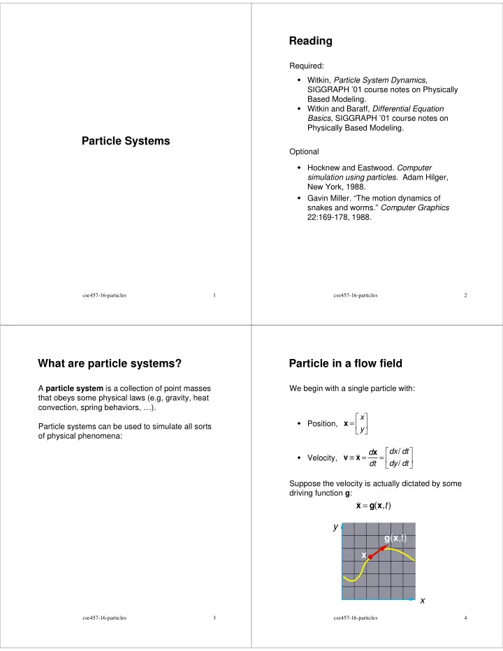
cse457-16-particles 3

What are particle systems?

A particle system is a collection of point masses that obeys some physical laws (e.g, gravity, heat convection, spring behaviors, …). Particle systems can be used to simulate all sorts

• f physical phenomena:

cse457-16-particles 4

Particle in a flow field

We begin with a single particle with: ! Position, ! Velocity, Suppose the velocity is actually dictated by some driving function g:

( , ) t = x g x &

/ / dx dt d dy dt dt   ≡ = =     x v x &

x g(x,t) x y

x y   =     x

cse457-16-particles 5

Vector fields

At any moment in time, the function g defines a vector field over x: How does our particle move through the vector field?

cse457-16-particles 6

Diff eqs and integral curves

The equation is actually a first order differential equation. We can solve for x through time by starting at an initial point and stepping along the vector field: This is called an intial value problem and the solution is called an integral curve.

Start Here

( , ) t = x g x &

cse457-16-particles 7

Euler’s method

One simple approach is to choose a time step, ∆t, and take linear steps along the flow: Writing as a time iteration: This approach is called Euler’s method and looks like: Properties: ! Simplest numerical method ! Bigger steps, bigger errors. Error ~ O(∆t2). Need to take pretty small steps, so not very

• efficient. Better (more complicated) methods exist,

e.g., “Runge-Kutta” and “implicit integration.”

+ ∆ ≈ + ∆ ⋅ ≈ + ∆ ⋅ & ( ) ( ) ( ) ( ) ( , ) t t t t t t t t x x x x g x

1 i i i

t

+ =

+ ∆ ⋅ x x v

cse457-16-particles 8

Particle in a force field

Now consider a particle in a force field f. In this case, the particle has: ! Mass, m ! Acceleration, The particle obeys Newton’s law: The force field f can in general depend on the position and velocity of the particle as well as time. Thus, with some rearrangement, we end up with:

( , , ) t m = f x x x & && m m = = f a x &&

2 2

d d dt dt ≡ = = v a x x &&

cse457-16-particles 9

This equation: is a second order differential equation. Our solution method, though, worked on first order differential equations. We can rewrite this as: where we have added a new variable v to get a pair

• f coupled first order equations.

Second order equations

( , , ) t m =       =   x v f x v v & & ( , , ) t m = f x v x &&

cse457-16-particles 10

Phase space

Concatenate x and v to make a 6- vector: position in phase space. Taking the time derivative: another 6-vector. A vanilla 1st-order differential equation.

      x v / m     =         x v v f & &       x v & &

cse457-16-particles 11

Differential equation solver

Applying Euler’s method:

( ) ( ) ( ) ( ) ( ) ( ) t t t t t t t t t t + ∆ = + ∆ ⋅ + ∆ = + ∆ ⋅ x x x x x x & & & &&

Again, performs poorly for large ∆t.

/ m     =         x v v f & &

+ +

= + ∆ ⋅ = + ∆ ⋅

1 1 i i i i i i

t t m x x v f v v

( ) ( ) ( ) ( , , ) ( ) ( ) t t t t t t t t t t m + ∆ = + ∆ ⋅ + ∆ = + ∆ ⋅ x x v f x x x x & & &

And making substitutions: Writing this as an iteration, we have: Starting with:

cse457-16-particles 12

Particle structure

m             x v f

position velocity force accumulator mass Position in phase space How do we represent a particle?

cse457-16-particles 13

Single particle solver interface

m             x v f       x v / m       v f

[ ]

6

getDim derivEval getState setState

cse457-16-particles 14

Particle systems

particles n time

In general, we have a particle system consisting

• f n particles to be managed over time:

                              L

1 2 1 2 1 2 1 2 n n n n

m m m x x x v v v f f f

cse457-16-particles 15

Particle system solver interface

particles n time L L

1 1 2 2 1 2 1 2 1 2

6

n n n n n

n m m m x v x v x v f f f v v v

derivEval get/setState getDim For n particles, the solver interface now looks like:

cse457-16-particles 16

Particle system diff. eq. solver

We can solve the evolution of a particle system again using the Euler method:

1 1 1 1 1 1 1 1 1 1 1

/ /

i i i i i i i i i n n n i i i n n n n

m t m

+ + + +

                        = + ∆                         x x v v v f x x v v v f M M M

cse457-16-particles 17

Forces

Each particle can experience a force which sends it on its merry way. Where do these forces come from? Some examples: ! Constant (gravity) ! Position/time dependent (force fields) ! Velocity-dependent (drag) ! N-ary (springs) How do we compute the net force on a particle?

cse457-16-particles 18

Particle systems with forces

particles n time forces F2 Fnf nf                               L

1 2 1 2 1 2 1 2 n n n n

m m m x x x v v v f f f

Force objects are black boxes that point to the particles they influence and add in their contributions. We can now visualize the particle system with force objects:

F1

cse457-16-particles 19

Gravity and viscous drag

grav

m = f G p->f += p->m * F->G

drag drag

k = − f v p->f -= F->k * p->v

The force due to gravity is simply: Often, we want to slow things down with viscous drag:

cse457-16-particles 20

A spring is a simple examples of an “N-ary” force. Recall the equation for the force due to a spring: We can augment this with damping: The resulting force equations become:

Damped spring

= − − ( )

spring

f k x r r = rest length

1 2

∆ = − x x x

1 1 1

p   =     x v

2 2 2

p   =     x v

= − − + [ ( ) ]

spring damp

f k x r k v     ∆ ⋅∆ ∆ = − ∆ − +     ∆ ∆       = −

1 2 1

( )

spring damp

k r k v x x f x x x f f

cse457-16-particles 21

               = = =                L

1 2 1 2 1 2 1 2 n n n n

m m m x x x v v v f f f

derivEval

• 1. Clear forces
• Loop over particles, zero force

accumulators

• 2. Calculate forces
• Sum all forces into accumulators
• 3. Return derivatives
• Loop over particles, return v and f/m

1 2 1 2 1 2 n n n

m m m                          v v v f f f L

Apply forces to particles Clear force accumulators

1 2 3

Return derivatives to solver

1 2 1 2 1 2 1 2 n n n n

m m m                               x x x v v v f f f L

F

2

F

3

Fnf F

1

cse457-16-particles 22

Bouncing off the walls

! Add-on for a particle simulator ! For now, just simple point-plane collisions

N P

A plane is fully specified by any point P on the plane and its normal N.

cse457-16-particles 23

Collision Detection

N v P x

How do you decide when you’ve crossed a plane?

cse457-16-particles 24

Normal and tangential velocity

( )

N T N

= ⋅ = − v N v N v v v

N

v N v P v

T

v

To compute the collision response, we need to consider the normal and tangential components

• f a particle’s velocity.

cse457-16-particles 25

Collision Response

before after

T restitution N

k = − ′ v v v

N

v v

T

v v’

resitution N

k − v

T

v

Without backtracking, the response may not be enough to bring a particle to the other side of a wall. In that case, detection should include a velocity check:

cse457-16-particles 26

Particle frame of reference

Let’s say we had our robot arm example and we wanted to launch particles from its tip. How would we go about starting the particles from the right place? First, we have to look at the coordinate systems in the OpenGL pipeline…

cse457-16-particles 27

The OpenGL geometry pipeline

cse457-16-particles 28

Projection and modelview matrices

Any piece of geometry will get transformed by a sequence of matrices before drawing: p’= Mproject Mview Mmodel p The first matrix is OpenGL’s GL_PROJECTION matrix. The second two matrices, taken as a product, are maintained on OpenGL’s GL_MODELVIEW stack: Mmodelview = Mview Mmodel

cse457-16-particles 29

Robot arm code, revisited

Recall that the code for the robot arm looked something like:

glRotatef( theta, 0.0, 1.0, 0.0 ); base(h1); glTranslatef( 0.0, h1, 0.0 ); glRotatef( phi, 0.0, 0.0, 1.0 ); upper_arm(h2); glTranslatef( 0.0, h2, 0.0 ); glRotatef( psi, 0.0, 0.0, 1.0 ); lower_arm(h3);

All of the GL calls here modify the modelview matrix. Note that even before these calls are made, the modelview matrix has been modified by the viewing transformation, Mview.

cse457-16-particles 30

Computing the particle launch point

To find the world coordinate position of the end of the robot arm, you need to follow a series of steps:

• 1. Figure out what Mview before drawing your model.
• 2. Draw your model and add one more transformation

to the tip of the robot arm. glTranslatef( 0.0, h3, 0.0 );

• 3. Compute
• 4. Transform a point at the origin by the resulting

matrix. Now you’re ready to launch a particle from that last computed point!

Vec3f particleOrigin = particleXform * Vec3f(0,0,0); Mat4f particleXform = ps->getWorldXform( matCam); Mat4f matCam = ps>glGetMatrix(GL_MODELVIEW_MATRIX);

=

• 1

model view modelview

M M M

cse457-16-particles 31

Summary

What you should take away from this lecture: ! The meanings of all the boldfaced terms ! Euler method for solving differential equations ! Combining particles into a particle system ! Physics of a particle system ! Various forces acting on a particle ! Simple collision detection ! How to hook your particle system into the coordinate frame of your model