Reading Jain, Kasturi, Schunck, Machine Vision . McGraw- Hill, 1995. - - PDF document

cse457-04-image-processing 1

Image processing

cse457-04-image-processing 2

Reading

Jain, Kasturi, Schunck, Machine Vision. McGraw- Hill, 1995. Sections 4.2-4.4, 4.5(intro), 4.5.5, 4.5.6, 5.1-5.4.

cse457-04-image-processing 3

What is an image?

We can think of an image as a function, f, from R2 to R: f( x, y ) gives the intensity of a channel at position ( x, y ) Realistically, we expect the image only to be defined over a rectangle, with a finite range:

• f: [a,b]x[c,d] [0,1]

A color image is just three functions pasted

• together. We can write this as a “vector-valued”

function:

( , ) ( , ) ( , ) ( , ) r x y f x y g x y b x y     =      

cse457-04-image-processing 4

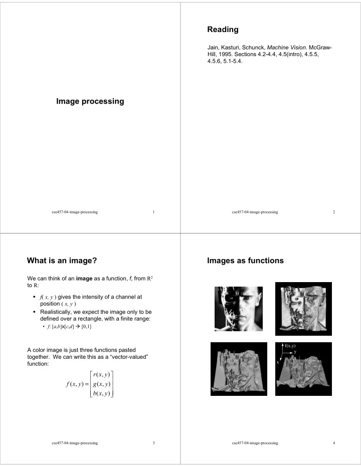
Images as functions

x y f(x,y)

What is a digital image?

In computer graphics, we usually operate on digital (discrete) images: Sample the space on a regular grid Quantize each sample (round to nearest integer) If our samples are ∆ apart, we can write this as: f[i ,j] = Quantize{ f(i ∆, j ∆) }

i j f[i,j] cse457-04-image-processing 6

Image processing

An image processing operation typically defines a new image g in terms of an existing image f. The simplest operations are those that transform each pixel in isolation. These pixel-to-pixel

• perations can be written:

Examples: RGB grayscale , threshold Note: a typical choice for mapping to grayscale is to apply the YIQ television matrix and keep the Y.

( , ) ( ( , )) g x y t f x y =

0.596 0.275 0.321 0.212 0.523 0.3 0.299 0.587 0.114 11 I Q Y R G B − − −           =               

cse457-04-image-processing 7

single pixel changes

to grayscale

⇒

threshold at 128 threshold at 55

cse457-04-image-processing 8

Pixel movement

Some operations preserve intensities, but move pixels around in the image Examples: many amusing warps of images

C

C

( , ) ( ( , ), ( , )) g x y f x x y y x y =

hair.ppt

cse457-04-image-processing 9

Pixel movement

Some operations preserve intensities, but move pixels around in the image

example: image registration

cse457-04-image-processing 10

More pixel movement effects

ripple image transitions reflection in ripples

Noise

Image processing is also useful for noise reduction and edge enhancement. We will focus on these applications for the remainder of the lecture… Common types of noise:

• Salt and pepper noise: contains random
• ccurrences of black and white pixels
• Impulse noise: contains random occurrences of

white pixels

• Gaussian noise: variations in intensity drawn

from a Gaussian normal distribution

cse457-04-image-processing 12

Ideal noise reduction

cse457-04-image-processing 13

Ideal noise reduction

cse457-04-image-processing 14

Practical noise reduction

Averaging multiple examples of the same image is often not possible. How can we “smooth” away noise in a single image? Is there a more abstract way to represent this sort

• f operation? Of course there is!

cse457-04-image-processing 15

Convolution

One of the most common methods for filtering an image is called convolution. In 1D, convolution is defined as: g(x) is “f convolved with h”

• ( )

( ) ( ) ( ') ( ') ' ( ') ( ' ) ' g x f x h x f x h x x dx f x h x x dx

∞ −∞ ∞ −∞

= ∗ = − = −

∫ ∫

x) h( (x) h − = ~ where

cse457-04-image-processing 16

cse457-04-image-processing 17

Discrete convolution

For a digital signal, we define discrete convolution as: g[i] is “f convolved with h”

• =

∗ = − = −

∑ ∑

' '

[ ] [ ] [ ] [ '] [ '] [ '] [ ' ]

i i

g i f i h i f i h i i f i h i i

] [ ] [ ~ where i h i h − =

cse457-04-image-processing 18 cse457-04-image-processing 19

Convolution in 2D

In two dimensions, convolution becomes: Similarly, discrete convolution in 2D becomes:

C[ , ]

[ , ] h i j h i j = − − where . ( , ) ( , ) ( , ) ( ', ') ( ', ') ' ' ( ', ') ( ' , ' ) ' ' g x y f x y h x y f x y h x x y y dx dy f x y h x x y y dx dy

∞ ∞ −∞ −∞ ∞ ∞ −∞ −∞

= ∗ = − − = − −

∫ ∫ ∫ ∫

( , )

( , ) h x y h x y = − − where .

∑∑ ∑∑

− − = − − = =

k l k l

j l i k h l k f l j k i h l k f j i h j i f j i g ] , [ ~ ] , [ ] , [ ] , [ ] , [ * ] , [ ] , [

cse457-04-image-processing 20

Convolution representation

Since f, g, and are defined over finite regions, we can write them out in two-dimensional arrays:

Note: This is not matrix multiplication!

h ~

242 245 245 245 244 228 191 165 245 246 240 220 204 184 151 138 232 192 165 141 131 142 138 136 190 165 144 143 142 140 137 138 141 145 148 146 135 135 135 135 0.2 0.2 0.2 0.2 0.2

f g

h ~

Q: What happens at the edges?

cse457-04-image-processing 21

Mean filters

How can we represent our noise-reducing averaging filter as a convolution diagram (know as a mean filter)?

cse457-04-image-processing 22

Effect of mean filters

cse457-04-image-processing 23

Gaussian filters

Gaussian filters weigh pixels based on their distance from the center of the convolution filter. In particular: This does a decent job of blurring noise while preserving features of the image. What parameter controls the width of the Gaussian? What happens to the image as the Gaussian filter kernel gets wider? What is the constant C? What should we set it to?

2 2 2

( )/(2 )

[ , ]

i j

e h i j C

σ − +

=

cse457-04-image-processing 24

Effect of Gaussian filters

cse457-04-image-processing 25

Median filters

A median filter operates over an mxm region by selecting the median intensity in the region. What advantage does a median filter have over a mean filter? Is a median filter a kind of convolution?

cse457-04-image-processing 26

Effect of median filters

cse457-04-image-processing 27

Comparison: Gaussian noise

cse457-04-image-processing 28

Comparison: salt and pepper noise

cse457-04-image-processing 29

Edge detection

One of the most important uses of image processing is edge detection: Really easy for humans Really difficult for computers Fundamental in computer vision Important in many graphics applications

cse457-04-image-processing 30

What is an edge?

Q: How might you detect an edge in 1D?

cse457-04-image-processing 31

Gradients

The gradient is the 2D equivalent of the derivative: Properties of the gradient It’s a vector Points in the direction of maximum increase

• f f

Magnitude is rate of increase How can we approximate the gradient in a discrete image?

( , ) , f f f x y x y   ∂ ∂ ∇ =    ∂ ∂

cse457-04-image-processing 32

Less than ideal edges

cse457-04-image-processing 33

Steps in edge detection

Edge detection algorithms typically proceed in three or four steps: Filtering: cut down on noise Enhancement: amplify the difference between edges and non-edges Detection: use a threshold operation Localization (optional): estimate geometry

• f edges beyond pixels

cse457-04-image-processing 34

Edge enhancement

A popular gradient magnitude computation is the Sobel operator: We can then compute the magnitude of the vector (sx, sy). 1 1 2 2 1 1 1 2 1 1 2 1

x y

s s −     = −     −       =     − − −  

Results of Sobel edge detection

cse457-04-image-processing 36

Second derivative operators

The Sobel operator can produce thick edges. Ideally, we’re looking for infinitely thin boundaries. An alternative approach is to look for local extrema in the first derivative: places where the change in the gradient is highest. Q: A peak in the first derivative corresponds to what in the second derivative?

cse457-04-image-processing 37

Localization with the Laplacian

An equivalent measure of the second derivative in 2D is the Laplacian: Using the same arguments we used to compute the gradient filters, we can derive a Laplacian filter to be: Zero crossings of this filter correspond to positions of maximum gradient. These zero crossings can be used to localize edges.

2 2 2 2 2

( , ) f f f x y x y ∂ ∂ ∇ = + ∂ ∂

2

1 1 4 1 1     ∆ = −      

cse457-04-image-processing 38

Localization with the Laplacian

Original Smoothed Laplacian (+128)

cse457-04-image-processing 39

Marching squares

We can convert these signed values into edge contours using a “marching squares” technique:

Sharpening with the Laplacian

Original Laplacian (+128) Original + Laplacian Original - Laplacian

Why does the sign make a difference? How can you write each filter that makes each bottom image?

cse457-04-image-processing 41

Summary

What you should take away from this lecture: The meanings of all the boldfaced terms. How noise reduction is done How discrete convolution filtering works The effect of mean, Gaussian, and median filters What an image gradient is and how it can be computed How edge detection is done What the Laplacian image is and how it is used in either edge detection or image sharpening