Reading Required: Angel 10.1-10.3, 10.5.2, 10.6-10.7 Optional - - PDF document

cse457-15-curves 1

Parametric curves

cse457-15-curves 2

Reading

Required: Angel 10.1-10.3, 10.5.2, 10.6-10.7 Optional Bartels, Beatty, and Barsky. An Introduction to Splines for use in Computer Graphics and Geometric Modeling, 1987.

• Farin. Curves and Surfaces for CAGD: A

Practical Guide, 4th ed., 1997.

cse457-15-curves 3

Curves before computers

The “loftsman’s spline”: long, narrow strip of wood or metal shaped by lead weights called “ducks” gives curves with second-order continuity, usually Used for designing cars, ships, airplanes, etc. But curves based on physical artifacts can’t be replicated well, since there’s no exact definition of what the curve is. Around 1960, a lot of industrial designers were working on this problem. Today, curves are easy to manipulate on a computer and are used for CAD, art, animation, …

cse457-15-curves 4

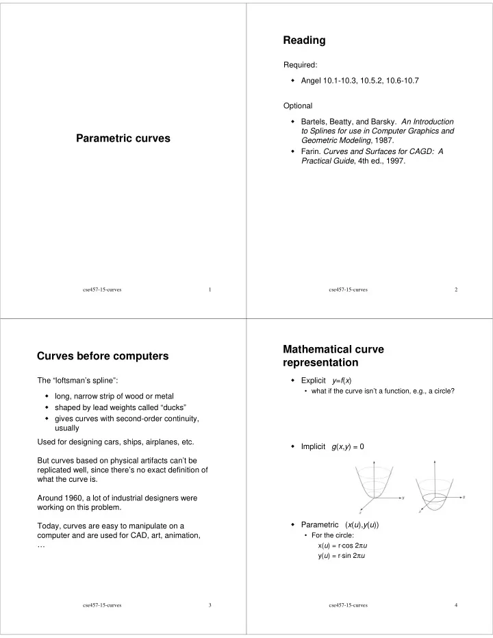
Mathematical curve representation

Explicit y=f(x)

• what if the curve isn’t a function, e.g., a circle?

Implicit g(x,y) = 0 Parametric (x(u),y(u))

• For the circle:

x(u) = r⋅cos 2πu y(u) = r⋅sin 2πu

cse457-15-curves 5

Parametric polynomial curves

We’ll use parametric curves, Q(u)=(x(u),y(u)), where the functions are all polynomials in the parameter. Advantages: easy (and efficient) to compute infinitely differentiable We’ll also assume that u varies from 0 to 1.

∑ ∑

= =

= =

n k k k n k k k

u b u y u a u x ) ( ) (

cse457-15-curves 6

Recursive interpolation: What if u=0? What if u=1?

de Casteljau’s algorithm

cse457-15-curves 7

Recursive notation: What is the equation for ?

de Casteljau’s algorithm, cont’d

1

V

cse457-15-curves 8

Finding Q(u)

Let’s solve for Q(u):

1 1 1 1 1 2 1 2 2 3 2 1 1 1 2 1 1 1 1 2 2 2 1 1 1 1 1 1 1 2 1 1 2 3 2 1

(1- ) (1- ) (1- ) (1- ) (1- ) ( ) (1- ) (1- )[(1- ) ] [(1- ) ] (1- )[(1- ){(1- ) } {(1- ) }] ... (1- ) 3 (1- ) V u V uV V u V uV V u V uV V u V uV V u V uV Q u u V uV u u V uV u u V uV u u u V uV u u V uV u V u u V = + = + = + = + = + = + = + + + = + + + + = +

2 3 2 3

3 (1- ) u u V u V + +

cse457-15-curves 9

Finding Q(u) (cont’d)

In general, where “n choose i” is: This defines a class of curves called Bézier curves. What’s the relationship between the number of control points and the degree of the polynomials?

( ) (1 )

n i n i i i

n Q u u u V i

− =

  = −    

∑

! ( )! ! n n i n i i   =     −

Bernstein polynomials

The coefficients of the control points are a set of functions called the Bernstein polynomials: For degree 3, we have: Useful properties on the interval [0,1]: each is between 0 and 1 sum of all four is exactly 1 (a.k.a., a “partition

• f unity”)

These together imply that the curve lies within the convex hull of its control points.

3 2 1 2 2 3 3

( ) (1 ) ( ) 3 (1 ) ( ) 3 (1 ) ( ) b u u b u u u b u u u b u u = − = − = − =

( ) ( )

n i i i

Q u b u V

=

=∑

cse457-15-curves 11

Displaying Bézier curves

How could we draw one of these things? It would be nice if we had an adaptive algorithm, that would take into account flatness.

DisplayBezier( V0, V1, V2, V3 ) begin if ( FlatEnough( V0, V1, V2, V3 ) ) Line( V0, V3 ); else something; end;

cse457-15-curves 12

Subdivide and conquer

DisplayBezier( V0, V1, V2, V3 ) begin if ( FlatEnough( V0, V1, V2, V3 ) ) Line( V0, V3 ); else Subdivide(V[]) ⇒ L[], R[] DisplayBezier( L0, L1, L2, L3 ); DisplayBezier( R0, R1, R2, R3 ); end;

cse457-15-curves 13

Testing for flatness

Compare total length of control polygon to length

• f line connecting endpoints:

1 1 2 2 3 3

1 V V V V V V V V ε − + − + − < + −

cse457-15-curves 14

Curve desiderata

Bézier curves offer a fairly simple way to model parametric curves. But, let’s consider some general properties we would like curves to have…

cse457-15-curves 15

Local control

One problem with Béziers is that every control point affects every point on the curve (except the endpoints). Moving a single control point affects the whole curve! We’d like to have local control, that is, have each control point affect some well-defined neighborhood around that point.

cse457-15-curves 16

Interpolation

Bézier curves are approximating. The curve does not (necessarily) pass through all the control

• points. Each point pulls the curve toward it, but
• ther points are pulling as well.

We’d like to have a curve that is interpolating, that is, that always passes through every control point.

cse457-15-curves 17

Continuity

We want our curve to have continuity: there shouldn’t be any abrupt changes as we move along the curve. There are nested degrees of continuity: C-1: C0: C1, C2 : C3, C4, …:

cse457-15-curves 18

Bézier curves

• splines

Bézier curves have C-infinity continuity on their interiors, but we saw that they do not exhibit local control or interpolate their control points. It is possible to define points that we want to interpolate, and then solve for the Bézier control points that will do the job. But, you will need as many control points as interpolated points -> high order polynomials -> wiggly curves. (And you still won’t have local control.) Instead, we’ll splice together a curve from individual Béziers segments, in particular, cubic Béziers. We call these curves splines. When splicing Béziers together, the first thing we need to worry about is continuity where one curve segment meets the next…

cse457-15-curves 19

Ensuring C0 continuity

Suppose we have a cubic Bézier defined by (V0,V1,V2,V3), and we want to attach another curve (W0,W1,W2,W3) to it, so that there is C0 continuity at the joint. What constraint(s) does this place on (W0,W1,W2,W3)?

=

0 :

(1 ) (0)

V W

C Q Q

cse457-15-curves 20

The C0 Bezier spline

How then could we construct a curve passing through a set of points P1…Pn? We call this curve a spline. The endpoints of the Bezier segments are called joints. In the animator project, you will construct such a curve by specifying all the Bezier control points directly.

cse457-15-curves 21

For degree 3 (cubic) curves, we have already shown that we get: We can expand the terms in u and rearrange to get: What then is the first derivative when evaluated at each endpoint, u=0 and u=1?

1st derivatives at the endpoints

= + + +

3 2 2 3 1 2 3

( ) (1- ) 3 (1- ) 3 (1- ) Q u u V u u V u u V u V = − + − + + − + + − + +

3 1 2 3 2 1 2 1

( ) ( 3 3 ) (3 6 3 ) ( 3 3 ) Q u V V V V u V V V u V V u V ′ = ′ = (0) (1 ) Q Q

cse457-15-curves 22

Ensuring C1 continuity

Suppose we have a cubic Bézier defined by (V0,V1,V2,V3), and we want to attach another curve (W0,W1,W2,W3) to it, so that there is C1 continuity at the joint. What constraint(s) does this place on (W0,W1,W2,W3)?

= =

1 ' '

: (1 ) (0) : (1 ) (0)

V W V W

C Q Q C Q Q

cse457-15-curves 23

The C1 Bezier spline

How then could we construct a curve passing through a set of points P1…Pn? We can specify the Bezier control points directly,

• r we can devise a scheme for placing them

automatically…

cse457-15-curves 24

Catmull-Rom splines

If we set each derivative to be one half of the vector between the previous and next controls, we get a Catmull-Rom spline. This leads to:

= = + = =

1 1 1 2 2 2 3 1 3 2

1 6 1 6

(

• )
• (
• )

V P V P P P V P P P V P

cse457-15-curves 25

We can give more control by exposing the derivative scale factor as a parameter: The parameter τ controls the tension. Catmull- Rom uses τ = 1/2. Here’s an example with τ =3/2.

Tension control

τ τ

= = + = =

1 1 1 2 2 2 3 1 3 2

3 3

(

• )
• (
• )

V P V P P P V P P P V P

cse457-15-curves 26

2nd derivatives at the endpoints

Finally, we’ll want to develop C2 splines. To do this, we’ll need second derivatives of Bezier curves. Taking the second derivative of Q(u) yields: ′′ = + = + ′′ = + = +

1 2 1 1 2 1 2 3 2 3 2 1

(0) 6(

• 2

)

• 6[(
• ) (
• )]

(1 ) 6(

• 2

)

• 6[(
• ) (
• )]

Q V V V V V V V Q V V V V V V V

cse457-15-curves 27

Ensuring C2 continuity

Suppose we have a cubic Bézier defined by (V0,V1,V2,V3), and we want to attach another curve (W0,W1,W2,W3) to it, so that there is C2 continuity at the joint. What constraint(s) does this place on (W0,W1,W2,W3)?

1 ' ' 2 '' ''

: (1 ) (0) : (1 ) (0) : (1 ) (0)

V W V W V W

C Q Q C Q Q C Q Q = = =

cse457-15-curves 28

Building a complex spline

Instead of specifying the Bézier control points themselves, let’s specify the corners of the A- frames in order to build a C2 continuous spline. These are called B-splines. The starting set of points are called de Boor points.

cse457-15-curves 29

B-splines

Here is the completed B-spline. What are the Bézier control points, in terms of the de Boor points?

1 1 2 1 2 1 1 2 2 1 2 3 1 2 3

____[____ ____ ] ____[____ ____ ] ____ ____ ____ ____ ____ ____ ____ ____ ____ ____ V B B B B B B B V B B V B B V B B B = + + + = + + = + = + = + +

cse457-15-curves 30

Endpoints of B-splines

We can see that B-splines don’t interpolate the de Boor points. It would be nice if we could at least control the endpoints of the splines explicitly. There’s a trick to make the spline begin and end at control points by repeating them. In the example below, let’s force interpolation of the last endpoint:

1 2 3 4 5

B B B B B B

cse457-15-curves 31

What if we want a closed curve, i.e., a loop? With Catmull-Rom and B-spline curves, this is easy:

Closing the loop

cse457-15-curves 32

In the animator project, you will draw a curve on the screen: You will actually treat this curve as: Where θ is a variable you want to animate. We can think of the result as a function: In general, you have to apply some constraints to make sure that θ(t) actually is a function.

Curves in the animator project

( )

= ( ) ( ), ( ) u x u y u Q θ = = ( ) ( ) ( ) ( ) u y u t u x u θ( ) t

cse457-15-curves 33

One of the extra credit options in the animator project is to implement “wrapping” so that the animation restarts smoothly when looping back to the beginning. This is a lot like making a closed curve: the calculations for the θ -coordinate are exactly the same. The t-coordinate is a little trickier: you need to create “phantom” t-coordinates before and after the first and last coordinates.

“Wrapping”

cse457-15-curves 34

Summary

What to take home from this lecture: Geometric and algebraic definitions of Bézier curves. Basic properties of Bézier curves. How to display Bézier curves with line segments. Meanings of Ck continuities. Geometric conditions for continuity of cubic splines. Properties of B-splines and Catmull-Rom splines. Geometric construction of B-splines and Catmull-Rom splines. How to construct closed loop splines.