1 Bezier Curve (with HW2 demo) Bezier Curve (with HW2 demo) Bezier - PDF document

Course Outline Course Outline Foundations of Computer Graphics Foundations of Computer Graphics  3D Graphics Pipeline (Spring 2012) (Spring 2012) CS 184, Lecture 12: Curves 1 Modeling Animation Rendering http://inst.eecs.berkeley.edu/~cs184 Graphics Pipeline Curves for Modeling Graphics Pipeline Curves for Modeling  In HW 1, HW 2, draw, shade objects  But how to define geometry of objects?  How to define, edit shape of teapot? 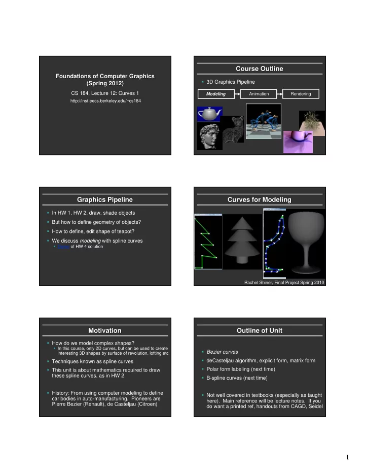 We discuss modeling with spline curves  Demo of HW 4 solution Rachel Shiner, Final Project Spring 2010 Motivation Motivation Outline of Unit Outline of Unit  How do we model complex shapes?  In this course, only 2D curves, but can be used to create  Bezier curves interesting 3D shapes by surface of revolution, lofting etc  deCasteljau algorithm, explicit form, matrix form  Techniques known as spline curves  Polar form labeling (next time)  This unit is about mathematics required to draw these spline curves, as in HW 2  B-spline curves (next time)  History: From using computer modeling to define  Not well covered in textbooks (especially as taught car bodies in auto-manufacturing. Pioneers are here). Main reference will be lecture notes. If you Pierre Bezier (Renault), de Casteljau (Citroen) do want a printed ref, handouts from CAGD, Seidel 1

Bezier Curve (with HW2 demo) Bezier Curve (with HW2 demo) Bezier Curve: (Desirable) properties Bezier Curve: (Desirable) properties  Interpolates, is tangent to end points  Motivation: Draw a smooth intuitive curve (or surface) given few key user-specified control points  Curve within convex hull of control polygon Control points (all that user specifies, edits) Control points (all that user specifies, edits) hw4.exe Control Control polygon polygon Smooth Bezier curve Smooth Bezier curve (drawn automatically) (drawn automatically) Issues for Bezier Curves deCasteljau: Linear Bezier Curve : Linear Bezier Curve Issues for Bezier Curves deCasteljau  Just a simple linear combination or interpolation Main question: Given control points and constraints (interpolation, tangent), how to construct curve? (easy to code up, very numerically stable) P1 F(1) Linear ( Degree 1, Order 2 )  Algorithmic: deCasteljau algorithm F(0) = P0, F(1) = P1 F(u) = ? F(u)  Explicit: Bernstein-Bezier polynomial basis P0 P0 P1  4x4 matrix for cubics F(0) 1-u u  Properties: Advantages and Disadvantages F(u) = (1-u) P0 + u P1 deCasteljau: Quadratic Bezier Curve : Quadratic Bezier Curve Geometric interpretation: Quadratic deCasteljau Geometric interpretation: Quadratic P1 Quadratic u Degree 2, Order 3 F(0) = P0, F(1) = P2 P2 1-u P0 F(u) = ? 1-u u P0 P1 P2 u 1-u u 1-u u 1-u u F(u) = (1-u) 2 P0 + 2u(1-u) P1 + u 2 P2 2

Geometric Interpretation: Cubic deCasteljau: Cubic Bezier Curve : Cubic Bezier Curve deCasteljau u P1 P2 Cubic Degree 3, Order 4 u F(0) = P0, F(1) = P3 u P3 P0 P0 P1 P2 P3 u 1-u u 1-u u u 1-u u 1-u u 1-u u u u 1-u F(u) = (1-u) 3 P0 +3u(1-u) 2 P1 +3u 2 (1-u) P2 + u 3 P3 Summary: deCasteljau deCasteljau Algorithm Algorithm DeCasteljau Implementation Implementation Summary: DeCasteljau P1 P1 P2 P1 P2 P0 P3 P0 P0 Linear Quadratic Cubic Degree 1, Order 2 Degree 2, Order 3 Degree 3, Order 4 F(0) = P0, F(1) = P1 F(0) = P0, F(1) = P2 F(0) = P0, F(1) = P3 P0 P1 P2 P0 P1 P2 P3 P0 P1 1-u u 1-u u 1-u u 1-u u 1-u u 1-u u 1-u u 1-u u 1-u u  Can be optimized to do without auxiliary storage F(u) = (1-u) P0 + u P1 F(u) = (1-u) 2 P0 + 2u(1-u) P1 + u 2 P2 1-u u F(u) = (1-u) 3 P0 +3u(1-u) 2 P1 +3u 2 (1-u) P2 + u 3 P3 Summary of HW2 Implementation Summary of HW2 Implementation Issues for Bezier Curves Issues for Bezier Curves Bezier (Bezier2 and Bspline discussed next time) Main question: Given control points and constraints  Arbitrary degree curve (number of control points) (interpolation, tangent), how to construct curve?  Break curve into detail segments. Line segments for these  Evaluate curve at locations 0, 1/detail, 2/detail, … , 1  Evaluation done using deCasteljau  Algorithmic: deCasteljau algorithm  Key implementation: deCasteljau for arbitrary degree  Is anyone confused? About handling arbitrary degree?  Explicit: Bernstein-Bezier polynomial basis  Can also use alternative formula if you want  Explicit Bernstein-Bezier polynomial form (next)  4x4 matrix for cubics  Properties: Advantages and Disadvantages  Questions? 3

Recap formulae Recap formulae Recap formulae Recap formulae  Linear combination of basis functions  Linear combination of basis functions       Linear: F u ( ) P (1 u ) Pu Linear: F u ( ) P (1 u ) Pu 0 1 0 1           2 2 2 2 Quadratic: F u ( ) P (1 u ) P [2 (1 u u )] P u Quadratic: F u ( ) P (1 u ) P [2 (1 u u )] P u 0 1 2 0 1 2               3 2 2 3 3 2 2 3 Cubic: F u ( ) P (1 u ) P [3 (1 u u ) ] P [3 u (1 u )] P u Cubic: F u ( ) P (1 u ) P [3 (1 u u ) ] P [3 u (1 u )] P u 0 1 2 3 0 1 2 3     n n Degree n: F u ( ) P B u ( ) Degree n: F u ( ) P B u ( ) k k k k k k n n B u ( ) areBernstein-Bezier polynomials B u ( ) areBernstein-Bezier polynomials k k  Explicit form for basis functions? Guess it?  Explicit form for basis functions? Guess it?  Binomial coefficients in [(1-u)+u] n Summary of Explicit Form Issues for Bezier Curves Summary of Explicit Form Issues for Bezier Curves Main question: Given control points and constraints    Linear: F u ( ) P (1 u ) Pu (interpolation, tangent), how to construct curve? 0 1      2 2 Quadratic: F u ( ) P (1 u ) P [2 (1 u u )] P u 0 1 2        3 2 2 3 Cubic: F u ( ) P (1 u ) P [3 (1 u u ) ] P [3 u (1 u )] P u 0 1 2 3  Algorithmic: deCasteljau algorithm    Explicit: Bernstein-Bezier polynomial basis n Degree n: F u ( ) P B u ( ) k k k  4x4 matrix for cubics n B u ( ) areBernstein-Bezier polynomials k  Properties: Advantages and Disadvantages n !    n n k k B u ( ) (1 u ) u  k !( )! k n k Cubic 4x4 Matrix (derive) Cubic 4x4 Matrix (derive) Cubic 4x4 Matrix (derive) Cubic 4x4 Matrix (derive)               3 2 2 3 3 2 2 3 F u ( ) P (1 u ) P [3 (1 u u ) ] P [3 u (1 u )] P u F u ( ) P (1 u ) P [3 (1 u u ) ] P [3 u (1 u )] P u 0 1 2 3 0 1 2 3           P 1 3 3 1 P 0 0             M ? P   3 6 3 0 P           1 1 3 2 3 2 u u u 1 u u u 1          P P 3 3 0 0    2     2    P   1 0 0 0  P  3 3 4

Issues for Bezier Curves Properties (brief discussion) Issues for Bezier Curves Properties (brief discussion)  Demo: Main question: Given control points and constraints hw4.exe (interpolation, tangent), how to construct curve?  Interpolation: End-points, but approximates others  Single piece, moving one point affects whole curve  Algorithmic: deCasteljau algorithm (no local control as in B-splines later)  Explicit: Bernstein-Bezier polynomial basis  Invariant to translations, rotations, scales etc. That is, translating all control points translates entire curve  4x4 matrix for cubics  Easily subdivided into parts for drawing (next lecture):  Properties: Advantages and Disadvantages Hence, Bezier curves easiest for drawing 5