Random Walk Example Values learned by TD(0) after various numbers - PDF document

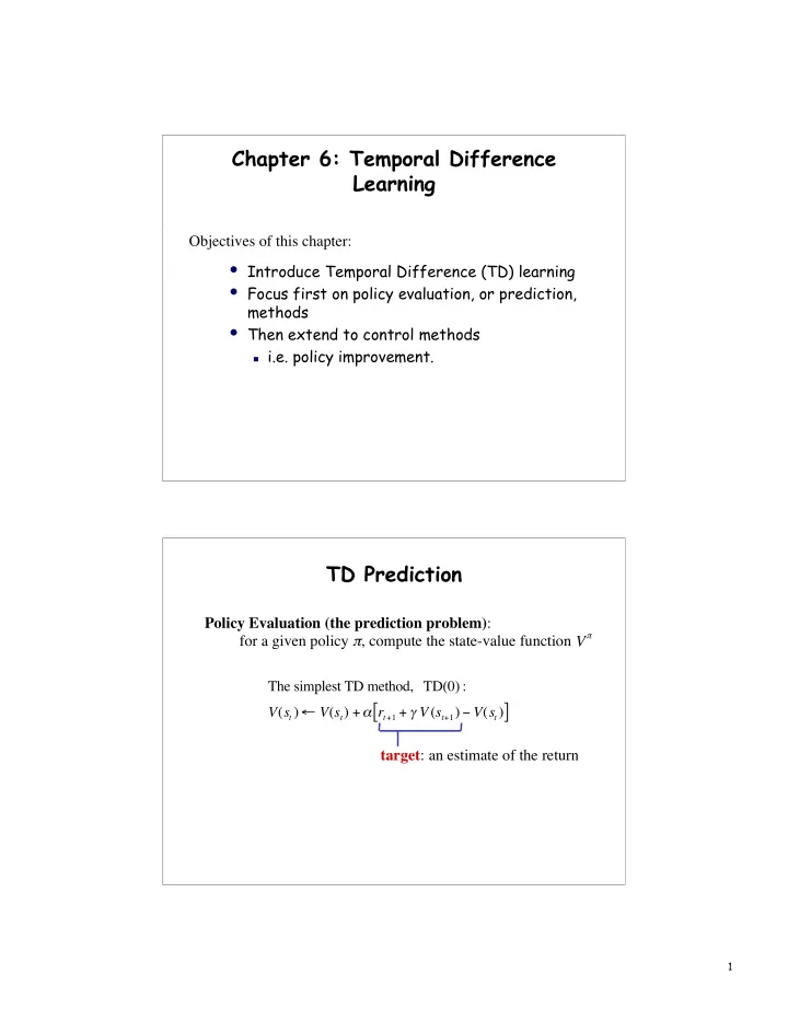
Chapter 6: Temporal Difference Learning Objectives of this chapter: • Introduce Temporal Difference (TD) learning • Focus first on policy evaluation, or prediction, methods • Then extend to control methods  i.e. policy improvement. TD Prediction Policy Evaluation (the prediction problem) : � for a given policy π , compute the state-value function V The simplest TD method, TD(0) : [ ] V ( s t ) � V ( s t ) + � r t + 1 + � V ( s t + 1 ) � V ( s t ) target : an estimate of the return 1

Simplest TD Method [ ] V ( s t ) � V ( s t ) + � r t + 1 + � V ( s t + 1 ) � V ( s t ) s t r t + 1 s t + 1 T T T T T T T T T T T T T T T T T T T T Advantages of TD Learning • TD methods do not require a model of the environment, only experience • TD methods can be fully incremental  You can learn before knowing the final outcome – Less memory – Less peak computation  You can learn without the final outcome – From incomplete sequences • TD converges to an optimal policy (under certain assumptions to be detailed later) 2

Random Walk Example Values learned by TD(0) after various numbers of episodes Optimality of TD(0) Batch Updating : train completely on a finite amount of data, e.g., train repeatedly on 10 episodes until convergence. Compute updates according to TD(0), but only update estimates after each complete pass through the data. For any finite Markov prediction task, under batch updating, TD(0) converges for sufficiently small α . 3

You are the Predictor Suppose you observe the following 8 episodes: A, 0, B, 0 B, 1 B, 1 V (A)? B, 1 B, 1 V (B)? B, 1 B, 1 B, 0 You are the Predictor V (A)? 4

You are the Predictor The prediction that best matches the training data is V(A)=0 •  This minimizes the mean-square-error on the training set • If we consider the sequentiality of the problem, then we would set V(A)=.75  This is correct for the maximum likelihood estimate of a Markov model generating the data  i.e, if we do a best fit Markov model, and assume it is exactly correct, and then compute what it predicts (how?)  This is called the certainty-equivalence estimate  This is what TD(0) gets Thought from Dan: If P(start at A) • is so low, apparently, who cares? Learning An Action-Value Function � for the current behavior policy � . Estimate Q After every transition from a nonterminal state s t , do this : ( ) � Q s t , a t ( ) + � r [ ( ) � Q s t , a t ( ) ] Q s t , a t t + 1 + � Q s t + 1 , a t + 1 If s t + 1 is terminal, then Q ( s t + 1 , a t + 1 ) = 0. 5

Sarsa: On-Policy TD Control Turn this into a control method by using the current greedy policy: One - step Sarsa : [ ] Q s t , a t ( ) � Q s t , a t ( ) + � r t + 1 + � Q s t + 1 , a t + 1 ( ) � Q s t , a t ( ) Q-Learning: Off-Policy TD Control One - step Q - learning : [ ] ( ) � Q s t , a t ( ) + � r ( ) � Q s t , a t ( ) Q s t , a t t + 1 + � max a Q s t + 1 , a 6

Cliffwalking ε− greedy , ε = 0.1 Summary • TD prediction • Introduced one-step tabular model-free TD methods • Extend prediction to control by employing some form of GPI  On-policy control: Sarsa  Off-policy control: Q-learning 7