Radiation Spectrum I Starting from the radiation field, we have - PowerPoint PPT Presentation

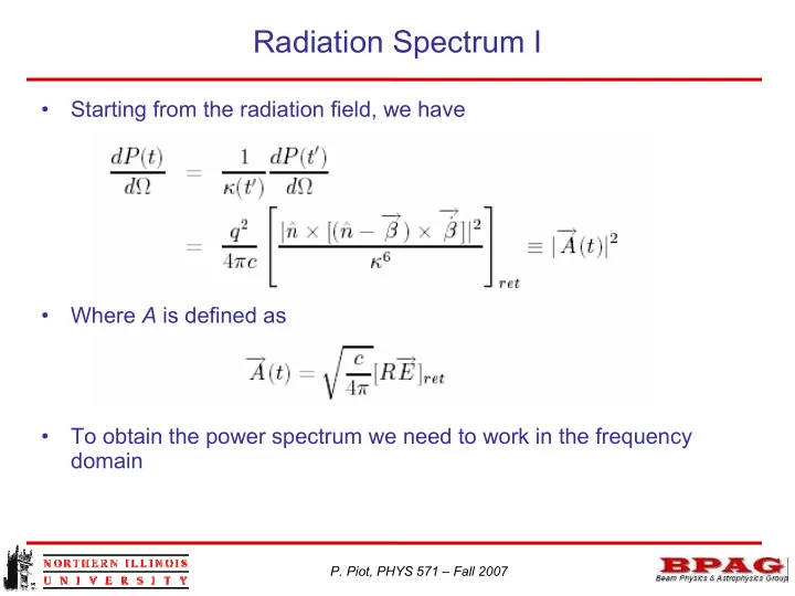
Radiation Spectrum I • Starting from the radiation field, we have • Where A is defined as • To obtain the power spectrum we need to work in the frequency domain P. Piot, PHYS 571 – Fall 2007

Radiation Spectrum II • Let’s define the “symmetrized Fourier transform” • Parseval’s theorem states that • Since A is a real function P. Piot, PHYS 571 – Fall 2007

Radiation Spectrum III • The radiation spectrum is therefore • Starting from A(t) A( ω ) is • P. Piot, PHYS 571 – Fall 2007

Radiation Spectrum IV • This must be evaluated at the retarded time t’ • Note that in the far-field regime is constant in time and argument of the exponential in the far-field is ignore ⇒ P. Piot, PHYS 571 – Fall 2007

Radiation Spectrum V • We finally have • And the corresponding angular spectral fluence distribution • This is the most general formula for computing the angular spectral fluence. • JDJ re-write the vector part of the integrand as a total time derivative P. Piot, PHYS 571 – Fall 2007

Radiation Spectrum VI • Consider • Then the time derivative is • We have P. Piot, PHYS 571 – Fall 2007

Radiation Spectrum VII • So we can do an integration-by-part =0 in principle but care must be taken to verify this in practice P. Piot, PHYS 571 – Fall 2007

Radiation Spectrum VIII • So finally the angular spectral fluence is note that • Here we could also start introducing the polarization, but we will do this for the special case of circular motion P. Piot, PHYS 571 – Fall 2007

Case of Circular motion I • Introduce the polarization unit y vectors ε ’s P ε ⊥ n ε || O θ x ω 0 t q r z • Then P. Piot, PHYS 571 – Fall 2007

Case of Circular motion II • The argument of the exponential writes If an observer catches an impulse from the charge q : θ is small and • the pulse originated close to t = 0 , so under these approximations and P. Piot, PHYS 571 – Fall 2007

Case of Circular motion III • The angular spectral fluence is σ π • This displays the two polarizations. P. Piot, PHYS 571 – Fall 2007

Case of Circular motion IV • We have to compute the integrals • We have P. Piot, PHYS 571 – Fall 2007

Case of Circular motion V • Finally the angular spectral fluence takes the form • …. P. Piot, PHYS 571 – Fall 2007

Case of Circular motion VI σ π σ π P. Piot, PHYS 571 – Fall 2007

Case of Circular motion VII σ+π P. Piot, PHYS 571 – Fall 2007