Quiz Question: Assuming a preemptive shortest job first algorithm is - - PowerPoint PPT Presentation

Quiz

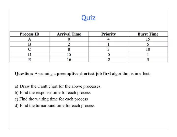
Question: Assuming a preemptive shortest job first algorithm is in effect, a) Draw the Gantt chart for the above processes. b) Find the response time for each process c) Find the waiting time for each process d) Find the turnaround time for each process

2

CSE 421/521 - Operating Systems Fall 2013

Tevfik Koşar

University at Buffalo

September 19th, 2013

Lecture - VI

CPU Scheduling - II

3

Roadmap

• CPU Scheduling

– Round-Robin Scheduling – Multilevel Feedback Queues – Estimating CPU bursts

4

Round Robin (RR)

• Each process gets a small unit of CPU time

(time quantum), usually 10-100 milliseconds. After this time has elapsed, the process is preempted and added to the end of the ready queue.

• If there are n processes in the ready queue and

the time quantum is q, then each process gets 1/n of the CPU time in chunks of at most q time units at once. No process waits more than (n-1)q time units.

• Performance

– q large ⇒ FIFO – q small ⇒ q must be large with respect to context switch, otherwise overhead is too high

Round Robin (RR)

5

A B C D E

Arrival times

RR (q = 1) scheduling policy

ü preemptive FCFS, based on a timeout interval, the quantum q ü the running process is interrupted by the clock and put last in a FIFO “Ready” queue; then, the first “Ready” process is run instead

A B C D E Mean

Stallings, W. (2004) Operating Systems: Internals and Design Principles (5th Edition).

Round Robin (RR)

6

A B C D E

Arrival times

RR (q = 4) scheduling policy

ü a crucial parameter is the quantum q (generally ~10–100ms) § q should be big compared to context switch latency (~10µs) § q should be less than the longest CPU bursts, otherwise RR degenerates to FCFS

A B C D E Mean

Stallings, W. (2004) Operating Systems: Internals and Design Principles (5th Edition).

7

Example of RR with Time Quantum = 20

Process Burst Time P1 53 P2

17

P3 68 P4

24

• For q=20, the Gantt chart is:

Typically, higher average turnaround than SJF , but better response

P1 P2 P3 P4 P1 P3 P4 P1 P3 P3 20 37 57 77 97 117 121 134 154 162

8

Time Quantum and Context Switch Time

9

Turnaround Time Varies With The Time Quantum

10

Comparison of Scheduling Algorithms

FCFS

PROS:

• It is a fair algorithm

– schedule in the order that they arrive

CONS:

• Average response time can be lousy

– small requests wait behind big ones

• May lead to poor utilization of other resources

– FCFS may result in poor overlap of CPU and I/O activity

• E.g., a CPU-intensive job prevents an I/O-intensive job from doing

a small bit of computation, thus preventing it from going back and keeping the I/O subsystem busy

11

SJF

PROS:

• Provably optimal with respect to average response time

– prevents convoy effect (long delay of short jobs)

CONS:

• Can cause starvation of long jobs
• Requires advanced knowledge of CPU burst times

– this can be very hard to predict accurately!

12

SJF

PROS:

• Guarantees early completion of high priority jobs

CONS:

• Can cause starvation of low priority jobs
• How to decide/assign priority numbers?

13

RR

PROS:

• Great for timesharing

– no starvation

• Does not require prior knowledge of CPU burst times

CONS:

• What if all jobs are almost time same length?
• How to set the “best” time quantum?

– if small, then context switch often, incurring high overhead – if large, then response time degrades

14

15

Multilevel Queue

• Ready queue is partitioned into separate queues:

foreground (interactive) background (batch)

• Each queue has its own scheduling algorithm

– foreground – RR – background – FCFS

• Scheduling must be done between the queues

– Fixed priority scheduling; (i.e., serve all from foreground then from background). Possibility of starvation. – Time slice – each queue gets a certain amount of CPU time which it can schedule amongst its processes; i.e., 80% to foreground in RR, 20% to background in FCFS

16

Multilevel Queues

17

Multilevel Queue Scheduling

18

Multilevel Feedback Queue

• A process can move between the various queues;

aging can be implemented this way

• Multilevel-feedback-queue scheduler defined by

the following parameters:

– number of queues – scheduling algorithms for each queue – method used to determine when to upgrade a process – method used to determine when to demote a process – method used to determine which queue a process will enter when that process needs service

19

Example of Multilevel Feedback Queue

• Three queues:

– Q0 – RR with time quantum 8 milliseconds – Q1 – RR time quantum 16 milliseconds – Q2 – FCFS

• Scheduling

– A new job enters queue Q0 which is served FCFS. When it gains CPU, job receives 8 milliseconds. If it does not finish in 8 milliseconds, job is moved to queue Q1. – At Q1 job is again served FCFS and receives 16 additional

• milliseconds. If it still does not complete, it is preempted and

moved to queue Q2.

20

Multilevel Feedback Queues

21

How to estimate CPU burst time?

22

Determining Length of Next CPU Burst

• Can only estimate the length
• Can be done by using the length of previous CPU bursts,

using exponential averaging

+

23

Examples of Exponential Averaging

• α =0

– τn+1 = τn – Recent history does not count

• α =1

– τn+1 = α tn – Only the actual last CPU burst counts

• If we expand the formula, we get:

τn+1 = α tn+(1 - α)α tn -1 + … +(1 - α )j α tn -j + … +(1 - α )n +1 τ0

• Since both α and (1 - α) are less than or equal to 1,

each successive term has less weight than its predecessor

24

Prediction of the Length of the Next CPU Burst

Alpha = 1/2, T0 = 10

Exercise

25

26

Summary

Hmm. .

• Next Lecture: Project-1 Discussion
• CPU Scheduling

– Round-Robin Scheduling – Multilevel Feedback Queues – Estimating CPU bursts

27

Acknowledgements

• “Operating Systems Concepts” book and supplementary

material by A. Silberschatz, P . Galvin and G. Gagne

• “Operating Systems: Internals and Design Principles”

book and supplementary material by W. Stallings

• “Modern Operating Systems” book and supplementary

material by A. Tanenbaum

• R. Doursat and M. Yuksel from UNR, Ed Lazowska from

UWashington