Quiz Define the vectors a 1 and a 2 as follows: a 1 = # $ % # $ - - PowerPoint PPT Presentation

Quiz

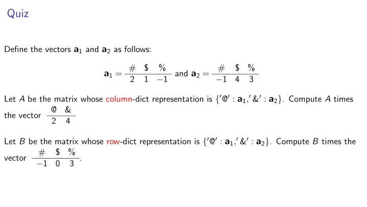
Define the vectors a1 and a2 as follows:

a1 = #

$ % 2 1 −1 and a2 = # $ % −1 4 3 Let A be the matrix whose column-dict representation is {0@0 : a1,0 &0 : a2}. Compute A times the vector @ & 2 4 Let B be the matrix whose row-dict representation is {0@0 : a1,0 &0 : a2}. Compute B times the vector # $ % −1 3 .

Matrices as vectors

Soon we study true matrix operations. But first.... A matrix can be interpreted as a vector:

I an R × S matrix is a function from R × S to F, I so it can be interpreted as an R × S-vector:

I scalar-vector multiplication I vector addition

I Our full implementation of Mat class will include these operations.

Transpose

Transpose swaps rows and columns. @ # ?

• a

| 2 1 3 b | 20 10 30 a b

• @

| 2 20 # | 1 10 ? | 3 30

Transpose (and Quiz)

Quiz: Write transpose(M) Answer: def transpose(M): return Mat((M.D[1], M.D[0]), {(q,p):v for (p,q),v in M.f.items()})

Computing sparse matrix-vector product

To compute matrix-vector or vector-matrix product,

I could use dot-product or linear-combinations definition. I However, using those definitions, it’s not easy to exploit sparsity in the matrix.

“Ordinary” Definition of Matrix-Vector Multiplication: If M is an R × C matrix and u is a C-vector then M ∗ u is the R-vector v such that, for each r ∈ R, v[r] = X

c2C

M[r, c]u[c]

Computing sparse matrix-vector product

“Ordinary” Definition of Matrix-Vector Multiplication: If M is an R × C matrix and u is a C-vector then M ∗ u is the R-vector v such that, for each r ∈ R, v[r] = X

c2C

M[r, c]u[c] Obvious method: 1 for i in R: 2 v[i] := P

j2C M[i, j]u[j]

But this doesn’t exploit sparsity! Idea:

I Initialize output vector v to zero vector. I Iterate over nonzero entries of M, adding terms according to ordinary definition.

1 initialize v to zero vector 2 for each pair (i, j) in sparse representation, 3 v[i] = v[i] + M[i, j]u[j]

Linear systems using matrices

Recall: A linear system is a system of linear equations

a1 · x

= β1 . . .

am · x

= βm Key idea: Write linear system as a matrix-vector equation. : 2 6 4

a1

. . .

am

3 7 5 x = b (((((

(

[β1, . . . , βm][β1, . . . , βm] We have many questions about linear systems:

I How to find a solution? I How many solutions?

I Does a solution even exist? I When does only one solution exist?

I What to do if there are no solutions? I For which right-hand sides β1, . . . , βm does

a solution exist? Matrices will help us answer these questions and use linear systems in other applications. First advantage of a matrix: Can interpret a row matrix as a column matrix: 2 4 v1 · · ·

vn

3 5 x = b Interpret this matrix-vector equation as: With what coefficients can b be written as a linear combination of v1, . . . , vn?

Linear systems using matrices

First advantage of a matrix: Can interpret a row matrix as a column matrix: 2 4 v1 · · ·

vn

3 5 x = b Interpret this matrix-vector equation as: With what coefficients can b be written as a linear combination of v1, . . . , vn? A solution to a Lights Out configuration is a linear combination of “button vectors.” For example, the linear combination

• =
• +

1

• +
• +

1

• can be written as
• =

2 6 6 4

• 3

7 7 5 ∗ [0, 1, 0, 1] Solving an instance of Lights Out ⇒ Solving a matrix-vector equation 2 3

Linear systems using matrices

A solution to a Lights Out configuration is a linear combination of “button vectors.” For example, the linear combination

• =
• +

1

• +
• +

1

• can be written as
• =

2 6 6 4

• 3

7 7 5 ∗ [0, 1, 0, 1] Solving an instance of Lights Out ⇒ Solving a matrix-vector equation

• =

2 6 6 4

• 3

7 7 5 ∗ [α1, α2, α3, α4]

The solver module

We provide a module solver that defines a procedure solve(A, b) that tries to find a solution to the matrix-vector equation A ∗ x = b Currently solve(A, b) is a black box but we will learn how to code it in the coming weeks. Let’s use it to solve this Lights Out instance...

The two fundamental spaces associated with a matrix

Want to study linear systems, equivalently matrix-vector equations Ax = b For which right-hand side vectors b does Ax = b have a solution? An R × C matrix A corresponds to the function f : FC − → FR defined by f (x) = Ax The system Ax = b has a solution if and only if there is some vector v such that Av = b. Thus the system has a solution if and only if there is some vector v in FC such that f (v) = b. Thus the system has a solution if and only if b is in the image of the function f . (Remember that the image of a function is the set of all possible outputs.) Question: How can we characterize the image of the function f (x) = Ax? Answer: Use the linear-combinations interpretation. For any input x, the output is the linear combination of the columns of A where coefficients are the entries of x. The set of all outputs is thus the set of all linear combinations of the columns of A. Also known as the span of the columns of A We call this the column space of A. Written Col A. We know it is a vector space.

The two fundamental spaces associated with a matrix

Recall: We are interested in solution set of corresponding homogeneous linear system 2 4 A 3 5 x = 0 We know this is a vector space. In context of matrices, we call it the null space of the matrix A. Written Null A Summary: The two most important spaces associated with a matrix A are

I Col A I Null A

Solution set of a matrix-vector equation

Proposition: If u1 is a solution to A ∗ x = b then solution set is u1 + V where V = Null A

I If V is a trivial vector space then u1 is the only solution. I If V is not trivial then u1 is not the only solution.

Corollary: A ∗ x = b has at most one solution iff Null A is a trivial vector space. Question: How can we tell if the null space of a matrix is trivial? Answer comes later...

Matrix-matrix multiplication

If

I A is a R × S matrix, and I B is a S × T matrix

then it is legal to multiply A times B.

I In Mathese, written AB I In our Mat class, written A*B

AB is different from BA. In fact, one product might be legal while the other is illegal.

Matrix-matrix multiplication: matrix-vector definition

Matrix-vector definition of matrix-matrix multiplication: For each column-label s of B, column s of AB = A ∗ (column s of B) Let A =  1 2 −1 1

• and

B = matrix with columns [4, 3], [2, 1], and [0, −1] B =  4 2 3 1 −1

• AB is the matrix with column i = A ∗ ( column i of B)

A ∗ [4, 3] = [10, −1] A ∗ [2, 1] = [4, −1] A ∗ [0, −1] = [−2, −1] AB =  10 4 −2 −1 −1 −1

Matrix-matrix multiplication: Dot-product definition

Combine

I matrix-vector definition of matrix-matrix multiplication, and I dot-product definition of matrix-vector multiplication

to get... Dot-product definition of matrix-matrix multiplication: Entry rc of AB is the dot-product of row r of A with column c of B. Example: 2 4 1 2 3 1 2 1 3 5 2 4 2 1 5 1 3 3 5 = 2 4 [1, 0, 2] · [2, 5, 1] [1, 0, 2] · [1, 0, 3] [3, 1, 0] · [2, 5, 1] [3, 1, 0] · [1, 0, 3] [2, 0, 1] · [2, 5, 1] [2, 0, 1] · [1, 0, 3] 3 5 = 2 4 4 7 11 3 5 5 3 5

Matrix-matrix multiplication: transpose

(AB)T = BTAT Example:  1 2 3 4  5 1 2

• =

 7 4 19 8

•  5

1 2 T  1 2 3 4 T =  5 1 2  1 3 2 4

• =

 7 19 4 8

• You might think “(AB)T = ATBT” but this is false.

In fact, doesn’t even make sense!

I For AB to be legal, A’s column labels = B’s row labels. I For ATBT to be legal, A’s row labels = B’s column labels.

Example: 2 4 1 2 3 4 5 6 3 5  6 7 8 9

• is legal but

 1 3 5 2 4 6  6 8 7 9

• is not.

Matrix-matrix multiplication: Column vectors

Multiplying a matrix A by a one-column matrix B 2 4 A 3 5 2 4 b 3 5 By matrix-vector definition of matrix-matrix multiplication, result is matrix with one column: A ∗ b This shows that matrix-vector multiplication is subsumed by matrix-matrix multiplication. Convention: Interpret a vector b as a one-column matrix (“column vector”)

I Write vector [1, 2, 3] as

2 4 1 2 3 3 5

I Write A ∗ [1, 2, 3] as

2 4 A 3 5 2 4 1 2 3 3 5 or A b