Quantum Marginal Problems David Gross (Colgone) Joint with: - - PowerPoint PPT Presentation

Quantum Marginal Problems

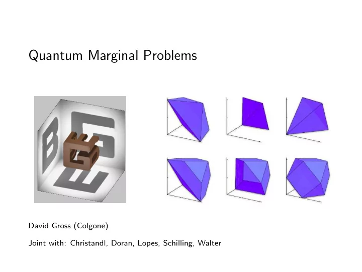
David Gross (Colgone) Joint with: Christandl, Doran, Lopes, Schilling, Walter

Outline

◮ Overview: Marginal problems ◮ Overview: Entanglement ◮ Main Theme: Entanglement Polytopes ◮ Shortly: Beyond the Pauli principle.

Overview: Marginal Problems

Marginals

◮ A marginal is obtained by

integrating out parts of high-dim

• bject

Marginals

◮ A marginal is obtained by

integrating out parts of high-dim

• bject

◮ Not every set of marginals is

compatible

Marginals

◮ A marginal is obtained by

integrating out parts of high-dim

• bject

◮ Not every set of marginals is

compatible

◮ Deciding compatibility is the

marginal problem

Marginals in classical probability

◮ Marginals are distributions of subsets of variables.

Marginals in classical probability

◮ Marginals are distributions of subsets of variables.

One classical marginal prob well-known in quantum:

Marginals in classical probability

◮ Marginals are distributions of subsets of variables.

One classical marginal prob well-known in quantum: Bell tests.

Bell tests as marginal problems

◮ There are four random variables:

polarization along two axes, as seen by Alice/Bob

Bell tests as marginal problems

◮ There are four random variables:

polarization along two axes, as seen by Alice/Bob

◮ Only certain pairs accessible ◮ Q: Are these marginals compatible with classical distribution?

Bell tests as marginal problems

◮ There are four random variables:

polarization along two axes, as seen by Alice/Bob

◮ Only certain pairs accessible ◮ Q: Are these marginals compatible with classical distribution? ◮ Compatible marginals form convex

polytope

◮ Facets are Bell inequalities.

Bell tests as marginal problems

◮ There are four random variables:

polarization along two axes, as seen by Alice/Bob

◮ Only certain pairs accessible ◮ Q: Are these marginals compatible with classical distribution? ◮ Compatible marginals form convex

polytope

◮ Facets are Bell inequalities. ◮ Testing locality NP-hard ⇒ so is classical marginal problem

Marginals in quantum theory

◮ For subset Si specify state ρi. ◮ Q: Are these compatible:

ρi = tr\Si ρ for some global ρ?

Marginals in quantum theory

◮ For subset Si specify state ρi. ◮ Q: Are these compatible:

ρi = tr\Si ρ for some global ρ? Would solve all finite-dim. few-body ground-state probs!

Marginals in quantum theory

◮ For subset Si specify state ρi. ◮ Q: Are these compatible:

ρi = tr\Si ρ for some global ρ? Would solve all finite-dim. few-body ground-state probs! E.g.: For two-body Hamiltonian H =

n

• i,j=1

hi,j, compute min

ρ trHρ = min ρ

• i,j

trhi,j ρ = min

{ρi,j} comp.

• i,j

trhi,j ρi,j.

Marginals in quantum theory: Ground States

min

ρ trHρ =

min

{ρi,j} comp.

• i,j

trhi,j ρi,j. Remarks:

◮ Left-hand side optimizes over O(dn) variables. ◮ R.h.s. over O(n2 d4). Exponential improvement!

Marginals in quantum theory: Ground States

min

ρ trHρ =

min

{ρi,j} comp.

• i,j

trhi,j ρi,j. Remarks:

◮ Left-hand side optimizes over O(dn) variables. ◮ R.h.s. over O(n2 d4). Exponential improvement! ◮ Optimization over convex set of compatible ρi,j.

Marginals in quantum theory: Ground States

min

ρ trHρ =

min

{ρi,j} comp.

• i,j

trhi,j ρi,j. Remarks:

◮ Left-hand side optimizes over O(dn) variables. ◮ R.h.s. over O(n2 d4). Exponential improvement! ◮ Optimization over convex set of compatible ρi,j.

General theory of convex optimization ⇒ Computational complexity of 2-RDM method (r.h.s) domi- nated by deciding compatibility of ρi,j’s.

Marginals in quantum theory: Ground States

min

ρ trHρ =

min

{ρi,j} comp.

• i,j

trhi,j ρi,j. Remarks:

◮ Left-hand side optimizes over O(dn) variables. ◮ R.h.s. over O(n2 d4). Exponential improvement! ◮ Optimization over convex set of compatible ρi,j.

General theory of convex optimization ⇒ Computational complexity of 2-RDM method (r.h.s) domi- nated by deciding compatibility of ρi,j’s. Two directions:

◮ Progress on q. marginal prob. ⇒ info about ground states ◮ Hardness of ground-states ⇒ hardness of q. marginals.

Negative direction

Computational complexity of 2-RDM method (r.h.s) domi- nated by deciding compatibility of ρi,j’s.

◮ But finding two-body ground-states is NP-hard ◮ (. . . and even QMA-hard)

Negative direction

Computational complexity of 2-RDM method (r.h.s) domi- nated by deciding compatibility of ρi,j’s.

◮ But finding two-body ground-states is NP-hard ◮ (. . . and even QMA-hard)

Thus: There is no efficient algorithm (quantum or classical) for the general two-body quantum marginal problem.

Negative direction

Computational complexity of 2-RDM method (r.h.s) domi- nated by deciding compatibility of ρi,j’s.

◮ But finding two-body ground-states is NP-hard ◮ (. . . and even QMA-hard)

Thus: There is no efficient algorithm (quantum or classical) for the general two-body quantum marginal problem.

◮ Remains hard for Fermions. ◮ Argument works for classical marginal prob. (hardness of Ising) ◮ Leaves room for outer approximations → D. Mazziotti’s talk.

Negative direction

Computational complexity of 2-RDM method (r.h.s) domi- nated by deciding compatibility of ρi,j’s.

◮ But finding two-body ground-states is NP-hard ◮ (. . . and even QMA-hard)

Thus: There is no efficient algorithm (quantum or classical) for the general two-body quantum marginal problem.

◮ Remains hard for Fermions. ◮ Argument works for classical marginal prob. (hardness of Ising) ◮ Leaves room for outer approximations → D. Mazziotti’s talk.

Natural Question: Is there subproblem with enough structure to be tractable?

1-RDM marginal problem

1-RDM subproblem: marginals do not overlap, global state pure

1-RDM marginal problem

1-RDM subproblem: marginals do not overlap, global state pure Classical version:

◮ Globally pure

⇔ no global randomness ⇒ no local randomness.

◮ . . . trivial.

1-RDM marginal problem

1-RDM subproblem: marginals do not overlap, global state pure Classical version:

◮ Globally pure

⇔ no global randomness ⇒ no local randomness.

◮ . . . trivial.

Quantum version:

◮ Globally pure

⇒ no local randomness (in presence of entanglement).

◮ . . . seems non-trivial, but tractable!

1-RDM marginal problem

Questions to be asked:

◮ Structure of set of 1-RDMs? ◮ What info about global ψ accessible from 1-RDM? ◮ Computational complexity of 1-RDM marginal prob.? ◮ Practical uses?

Structure of 1-RDMs.

Reduction to eigenvalues

◮ Local basis change does not affect compatibility ◮ ⇒ can assume ρi are diagonal ⇒ described by eigenvalues

• λ(1), . . . ,

λ(n) ∈ ❘dn.

Reduction to eigenvalues

◮ Local basis change does not affect compatibility ◮ ⇒ can assume ρi are diagonal ⇒ described by eigenvalues

• λ(1), . . . ,

λ(n) ∈ ❘dn. Question becomes: Which set of ordered local eigenvalues λ(i) can occur?

Reduction to eigenvalues

◮ Local basis change does not affect compatibility ◮ ⇒ can assume ρi are diagonal ⇒ described by eigenvalues

• λ(1), . . . ,

λ(n) ∈ ❘dn. Question becomes: Which set of ordered local eigenvalues λ(i) can occur? Deep fact:

◮ Compatible spectra form convex polytope

Reduction to eigenvalues

◮ Local basis change does not affect compatibility ◮ ⇒ can assume ρi are diagonal ⇒ described by eigenvalues

• λ(1), . . . ,

λ(n) ∈ ❘dn. Question becomes: Which set of ordered local eigenvalues λ(i) can occur? Deep fact:

◮ Compatible spectra form convex polytope ◮ Highly non-trivial! (Global set is not convex).

Reduction to eigenvalues

◮ Local basis change does not affect compatibility ◮ ⇒ can assume ρi are diagonal ⇒ described by eigenvalues

• λ(1), . . . ,

λ(n) ∈ ❘dn. Question becomes: Which set of ordered local eigenvalues λ(i) can occur? Deep fact:

◮ Compatible spectra form convex polytope ◮ Highly non-trivial! (Global set is not convex). ◮ Several proofs, building on symplectic

geometry & asymptotic rep theory

[Klyachko, Kirwan, Christandl, Mitchison, Harrow, Daftuar, Hayden, . . . ]

Reduction to eigenvalues

◮ Local basis change does not affect compatibility ◮ ⇒ can assume ρi are diagonal ⇒ described by eigenvalues

• λ(1), . . . ,

λ(n) ∈ ❘dn. Question becomes: Which set of ordered local eigenvalues λ(i) can occur? Deep fact:

◮ Compatible spectra form convex polytope ◮ Highly non-trivial! (Global set is not convex). ◮ Several proofs, building on symplectic

geometry & asymptotic rep theory

[Klyachko, Kirwan, Christandl, Mitchison, Harrow, Daftuar, Hayden, . . . ] ◮ No conceptually simple proof known to me!

Example: d = n = 2

Warm up: work out solution for two qubits.

Example: d = n = 2

Warm up: work out solution for two qubits.

◮ Schmidt-decomposition:

|ψ =

• λ(1)|e1 ⊗ |f1 +
• λ(2)|e2 ⊗ |f2

◮ With

ρ1 = λ(1)|e1e1|+λ(2)|e2e2|, ρ2 = λ(1)|f1f1|+λ(2)|f2f2|.

Example: d = n = 2

Warm up: work out solution for two qubits.

◮ Schmidt-decomposition:

|ψ =

• λ(1)|e1 ⊗ |f1 +
• λ(2)|e2 ⊗ |f2

◮ With

ρ1 = λ(1)|e1e1|+λ(2)|e2e2|, ρ2 = λ(1)|f1f1|+λ(2)|f2f2|.

◮ So eigenvalues must be equal:

λ1 = λ2.

Example: d = n = 2

Warm up: work out solution for two qubits.

◮ Schmidt-decomposition:

|ψ =

• λ(1)|e1 ⊗ |f1 +
• λ(2)|e2 ⊗ |f2

◮ With

ρ1 = λ(1)|e1e1|+λ(2)|e2e2|, ρ2 = λ(1)|f1f1|+λ(2)|f2f2|.

◮ So eigenvalues must be equal:

λ1 = λ2. In terms of largest eigenvalue, get simple polytope:

Further examples

Three qubits: Three fermions on 6 modes (“Dennis-Borland”): (c.f. M. Christandl’s talk)

Summary: Structure of 1-RDM’s

◮ Compatible 1-RDMs described by convex polytopes of spectra.

Summary: Structure of 1-RDM’s

◮ Compatible 1-RDMs described by convex polytopes of spectra. ◮ If this doesn’t surprise you, I’m terribly sad.

Computational aspects.

List inequalities?

[Klyachko, Altunbulak] ◮ Polytopes characterized by finitely

many linear ineqs D, x ≤ c.

List inequalities?

[Klyachko, Altunbulak] ◮ Polytopes characterized by finitely

many linear ineqs D, x ≤ c.

◮ Ansatz so far: Compute all ineqs → Altunbulak’s talk ◮ Doesn’t seem to scale: too many ineqs

as n, d go up.

List inequalities?

[Klyachko, Altunbulak] ◮ There might be better algorithm than

“checking all ineqs”. ❘

List inequalities?

[Klyachko, Altunbulak] ◮ There might be better algorithm than

“checking all ineqs”.

◮ Ex.: ℓ1-unit ball in ❘n has 2n linear

ineqs, but membership equivalent to xℓ1 =

n

• i=1

|xi| ≤ 1.

Computational complexity

Thus, central open question: Q.: Is there a poly-time algorithm that decides the 1-RDM quantum marginal problem?

Computational complexity

Thus, central open question: Q.: Is there a poly-time algorithm that decides the 1-RDM quantum marginal problem? Progress Nov. 2015 [Burgisser, Christandl, Mulmuley, Walter]: Problem in NP ∩ coNP

◮ Virtually guarantees that it can’t be proven hard ◮ Suggests it might be in P.

Info about global state from 1-RDMs. Part 1: Selection rules.

Selection rules

Selection rule, “Generalized Hartree-Fock”: If a state ψ maps to the boundary of the polytope, only few, special Slater determinants can appear in an expansion of ψ.

v

(a)

v

(b)

v

(c)

v

(d)

Selection rules

Selection rule, “Generalized Hartree-Fock”: If a state ψ maps to the boundary of the polytope, only few, special Slater determinants can appear in an expansion of ψ.

◮ Stated by Klyachko (2009). He

didn’t feel proof was necessary.

◮ True for for general scenarios –

stated here for Fermions.

v

(a)

v

(b)

v

(c)

v

(d)

[Schilling, DG, Christandl, PRL ’13]

Selection rules

◮ Consider n-Fermion system with modes {φ1, . . . , φd}.

Selection rules

◮ Consider n-Fermion system with modes {φ1, . . . , φd}. ◮ Expand ψ ∈ ∧nCd in Slater dets:

ψ =

• i1<···<in

ci1,...,in φi1 ∧ · · · ∧ φin. (1)

Selection rules

◮ Consider n-Fermion system with modes {φ1, . . . , φd}. ◮ Expand ψ ∈ ∧nCd in Slater dets:

ψ =

• i1<···<in

ci1,...,in φi1 ∧ · · · ∧ φin. (1)

◮ Assume (wlog) ρ(1)(ψ) is diagonal with eigenvalues λ

Selection rules

◮ Consider n-Fermion system with modes {φ1, . . . , φd}. ◮ Expand ψ ∈ ∧nCd in Slater dets:

ψ =

• i1<···<in

ci1,...,in φi1 ∧ · · · ∧ φin. (1)

◮ Assume (wlog) ρ(1)(ψ) is diagonal with eigenvalues λ ◮ Let D, x ≤ c be a face of the 1-RDM polytope.

Selection rules

◮ Consider n-Fermion system with modes {φ1, . . . , φd}. ◮ Expand ψ ∈ ∧nCd in Slater dets:

ψ =

• i1<···<in

ci1,...,in φi1 ∧ · · · ∧ φin. (1)

◮ Assume (wlog) ρ(1)(ψ) is diagonal with eigenvalues λ ◮ Let D, x ≤ c be a face of the 1-RDM polytope.

If the eigenvalues of ψ saturate the ineq. D, λ = c, then (1)

• nly contains Slater dets whose eigenvalues do so as well.

Selection rules: Proof

If the eigenvalues of ψ saturate the ineq. D, λ = c, then (1)

• nly contains Slater dets whose eigenvalues do so as well.

Elementary proof [Alex Lopes, PhD thesis; Lopes, Schilling, DG, in eternal prep.]

Selection rules: Proof

If the eigenvalues of ψ saturate the ineq. D, λ = c, then (1)

• nly contains Slater dets whose eigenvalues do so as well.

Elementary proof [Alex Lopes, PhD thesis; Lopes, Schilling, DG, in eternal prep.] Trick:

◮ Introduce operator ˆ

D =

i Di a† i ai. ◮ Then

D, λ = tr ˆ Dρ(1) = tr ˆ D|ψψ|.

Selection rules: Proof

If the eigenvalues of ψ saturate the ineq. D, λ = c, then (1)

• nly contains Slater dets whose eigenvalues do so as well.

Elementary proof [Alex Lopes, PhD thesis; Lopes, Schilling, DG, in eternal prep.] Trick:

◮ Introduce operator ˆ

D =

i Di a† i ai. ◮ Then

D, λ = tr ˆ Dρ(1) = tr ˆ D|ψψ|. Selection rule equivalent to: If tr ˆ D|ψψ| = c, then ˆ D|ψ = c|ψ. (Non-trivial, as c need not be extremal eigenvalue of ˆ D).

Selection rules: Proof

If the eigenvalues of ψ saturate the ineq. D, λ = c, then (1)

• nly contains Slater dets whose eigenvalues do so as well.

Elementary proof [Alex Lopes, PhD thesis; Lopes, Schilling, DG, in eternal prep.] Trick:

◮ Introduce operator ˆ

D =

i Di a† i ai. ◮ Then

D, λ = tr ˆ Dρ(1) = tr ˆ D|ψψ|. Selection rule equivalent to: If tr ˆ D|ψψ| = c, then ˆ D|ψ = c|ψ. (Non-trivial, as c need not be extremal eigenvalue of ˆ D). Proof: Blackboard.

Info about global state from 1-RDMs. Part 2: Entanglement.

Entanglement

◮ Two pure states ψ, φ are in same entanglement class if they

can be converted into each other with finite probability of success using local operations and classical communication. ❈ ❈

Entanglement

◮ Two pure states ψ, φ are in same entanglement class if they

can be converted into each other with finite probability of success using local operations and classical communication.

◮ Often referred to as SLOCC classes. But that sounds too

unpleasant. ❈ ❈

Entanglement

◮ Two pure states ψ, φ are in same entanglement class if they

can be converted into each other with finite probability of success using local operations and classical communication.

◮ Often referred to as SLOCC classes. But that sounds too

unpleasant.

◮ Formally:

ψ ∼ φ ⇔ ψ = (g1 ⊗ · · · ⊗ gn)φ with gi local invertible matrices (filtering operations).

◮ Mathematically: We’re looking at SL(❈d)×n-orbits in

• ❈dn.

SLOCC, SLOCC! – Who’s There?

◮ For three qubits (d = 2, n = 3), equivalence classes known

since mid-1800s. Re-discovered in 2000 to great effect:

Examples

Classes:

◮ Products ψ = φ1 ⊗ φ2 ⊗ φ3. ◮ Three classes of bi-separable states: ψ = φ1 ⊗ φ2,3. ◮ The W-class:

|W = |001 + |010 + |100.

◮ The GHZ-class:

|GHZ = |000 + |111.

Further examples

4 qubits:

◮ Classification apparently first obtained in QI community

[Verstraete et al. (2002)].

◮ Nine families of four complex parameters each.

Further examples

4 qubits:

◮ Classification apparently first obtained in QI community

[Verstraete et al. (2002)].

◮ Nine families of four complex parameters each.

Beyond:

◮ Number of parameters required to label orbits increases

exponentially.

◮ Only sporadic facts known.

Desiderata

Can we come up with theory that

◮ is systematic

(any number of particles, local dimensions, symmetry constraints),

◮ is efficient

(only polynomial number of parameters have to be learned),

◮ experimentally feasible

(parameters easily accessible, robust to noise)?

Desiderata

Can we come up with theory that

◮ is systematic

(any number of particles, local dimensions, symmetry constraints),

◮ is efficient

(only polynomial number of parameters have to be learned),

◮ experimentally feasible

(parameters easily accessible, robust to noise)? Claim: The single-site quantum marginal problem lives up to these standards.

Entanglement Polytopes

Central observation, entanglement polytopes

Set of allowed eigenvalues may depend on entanglement class

• f global state.

Central observation, entanglement polytopes

Set of allowed eigenvalues may depend on entanglement class

• f global state.

Thus:

◮ To every class C, associated set ∆C of local eigenvalues of

states in (closure of) C.

Central observation, entanglement polytopes

Set of allowed eigenvalues may depend on entanglement class

• f global state.

Thus:

◮ To every class C, associated set ∆C of local eigenvalues of

states in (closure of) C.

◮ Turns out: ∆C is again polytope: the entanglement polytope

associated with C.

[Walter, Doran, Gross, Christandl, Science 2013]

Central observation, entanglement polytopes

Set of allowed eigenvalues may depend on entanglement class

• f global state.

Thus:

◮ To every class C, associated set ∆C of local eigenvalues of

states in (closure of) C.

◮ Turns out: ∆C is again polytope: the entanglement polytope

associated with C.

[Walter, Doran, Gross, Christandl, Science 2013] ◮ Clearly: the position of

λ(ψ) w.r.t. the entanglement polytopes contains all local information about global entanglement class.

Examples re-visited: 3 qubit entanglement polytopes

For three qubits, polytopes resolve all 6 entanglement classes: [Hang et al. (2004), Sawicki et al. (2012), our paper]

Examples re-visited: 3 qubit entanglement polytopes

For three qubits, polytopes resolve all 6 entanglement classes: [Hang et al. (2004), Sawicki et al. (2012), our paper] W-class corresponds to “upper pyramid”: λ(1)

max + λ(2) max + λ(3) max ≥ 2.

Any violation of that witnesses GHZ-type entanglement.

Examples re-visited: 4 qubit entanglement polytopes

4 qubits:

◮ Entanglement classes:

9 families with up to four complex parameters each [Verstraete et al. (2002)].

Examples re-visited: 4 qubit entanglement polytopes

4 qubits:

◮ Entanglement classes:

9 families with up to four complex parameters each [Verstraete et al. (2002)].

◮ Entanglement Polytopes:

13 polytopes, 7 of which are genuinely 4-party entangled.

Examples re-visited: 4 qubit entanglement polytopes

4 qubits:

◮ Entanglement classes:

9 families with up to four complex parameters each [Verstraete et al. (2002)].

◮ Entanglement Polytopes:

13 polytopes, 7 of which are genuinely 4-party entangled.

◮ We feel: attractive balance between coarse-graining and

preserving structure. Example: 4-qubit W-class CW ∋ |0001 + |0010 + |0100 + |1000 again an “upper pyramid”: λ(1)

max + λ(2) max + λ(3) max + λ(4) max ≥ 3.

Example: 4 qubit entanglement polytopes

Example: Bosonic qubits

Consider n bosonic qubits: ψ ∈ Symn ❈2 .

Example: Bosonic qubits

Consider n bosonic qubits: ψ ∈ Symn ❈2 .

◮ Symmetry ⇒ all local reductions are equal:

ρ(1)

i,j = ψ|a† i aj|ψ. ◮ ⇒ single number captures all: λmax ∈ [0.5, 1].

Example: Bosonic qubits

Consider n bosonic qubits: ψ ∈ Symn ❈2 .

◮ Symmetry ⇒ all local reductions are equal:

ρ(1)

i,j = ψ|a† i aj|ψ. ◮ ⇒ single number captures all: λmax ∈ [0.5, 1].

Analyze polytopes:

◮ |0, . . . , 0 in all C’s ⇒ ∆C = [γC, 1].

Example: Bosonic qubits

Consider n bosonic qubits: ψ ∈ Symn ❈2 .

◮ Symmetry ⇒ all local reductions are equal:

ρ(1)

i,j = ψ|a† i aj|ψ. ◮ ⇒ single number captures all: λmax ∈ [0.5, 1].

Analyze polytopes:

◮ |0, . . . , 0 in all C’s ⇒ ∆C = [γC, 1]. ◮ Turns out: Possible choices are

γC ∈ 1 2

• ∪

N − k N : k = 0, 1, . . . , ⌊N/2⌋

• . . .

◮ . . . with innermost point γ the image of W -type states.

Example: No Solipsism

◮ A vector is genuinely n-partite entangled if it does not

factorize w.r.t. any bi-partition: ψ = ψ1 ⊗ ψ2.

Example: No Solipsism

◮ A vector is genuinely n-partite entangled if it does not

factorize w.r.t. any bi-partition: ψ = ψ1 ⊗ ψ2. Observation: sometimes detectable from local spectra alone.

Example: No Solipsism

◮ A vector is genuinely n-partite entangled if it does not

factorize w.r.t. any bi-partition: ψ = ψ1 ⊗ ψ2. Observation: sometimes detectable from local spectra alone. ⇔ spectra ( λ(1), . . . , λ(n)) compatible, but no bi-partition is. Example: (λ(1)

max, . . . , λ(n) max) =

1 2 + 1 n − 1, 1 − 1 n − 1, . . . , 1 − 1 n − 1

• .

Example: No Solipsism

◮ A vector is genuinely n-partite entangled if it does not

factorize w.r.t. any bi-partition: ψ = ψ1 ⊗ ψ2. Observation: sometimes detectable from local spectra alone. ⇔ spectra ( λ(1), . . . , λ(n)) compatible, but no bi-partition is. Example: (λ(1)

max, . . . , λ(n) max) =

1 2 + 1 n − 1, 1 − 1 n − 1, . . . , 1 − 1 n − 1

• .

Interpretation:

◮ no solipsism: love needs a partner!

(And entangled qubits need their counter-parts).

Example: Distillation

Entanglement measures from local information:

◮ (Linear) entropy of entanglement

E(ψ) = 1 − 1 N

• i

trρ2

i

simple function of Euclidean distance of eigenvalue point to origin.

◮ “Closer to origin ⇒ more entanglement”.

Example: Distillation

Entanglement measures from local information:

◮ (Linear) entropy of entanglement

E(ψ) = 1 − 1 N

• i

trρ2

i

simple function of Euclidean distance of eigenvalue point to origin.

◮ “Closer to origin ⇒ more entanglement”. ◮ ⇒ can bound distillable entanglement from local information!

Example: Distillation

Entanglement measures from local information:

◮ (Linear) entropy of entanglement

E(ψ) = 1 − 1 N

• i

trρ2

i

simple function of Euclidean distance of eigenvalue point to origin.

◮ “Closer to origin ⇒ more entanglement”. ◮ ⇒ can bound distillable entanglement from local information! ◮ Can even give distillation procedure without need to know

state beyond local densities (generalizing [Verstraete et al. 2002]).

Pure???

◮ Yeah, but no pure state exists in Nature.

Pure???

◮ Yeah, but no pure state exists in Nature. ◮ Results are epsilonifiable: if distance d of spectrum to a

polytope ∆ exceeds 4N

• 1 − p,

then ρ ∈ conv(∆).

◮ p = tr ρ2 is purity, which an be lower-bounded from local

information alone.

Summary of Entanglement Polytopes

◮ Locally accessible info about global entanglement encoded in

entanglement polytopes – subpolytopes of the set of admissible local spectra.

◮ Provides a systematic and efficient way of obtaining

information about entanglement classes.

Thank you for your attention!

David Gross (Uni Cologne) Oxford, April 2016