
SLIDE 1
Pythagoras Theorem in Noncommutative Geometry
Francesco D’Andrea
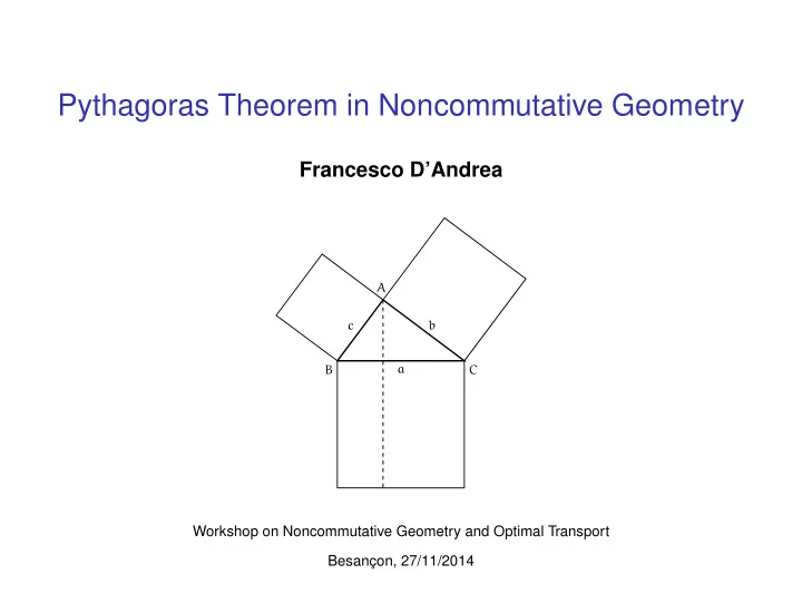
A B C c a b
Workshop on Noncommutative Geometry and Optimal Transport Besanc ¸on, 27/11/2014
Pythagoras Theorem in Noncommutative Geometry Francesco DAndrea A - - PowerPoint PPT Presentation
Pythagoras Theorem in Noncommutative Geometry Francesco DAndrea A c b B a C Workshop on Noncommutative Geometry and Optimal Transport Besanc on, 27/11/2014 Introduction The line element in nc geometry is the inverse of the
A B C c a b
Workshop on Noncommutative Geometry and Optimal Transport Besanc ¸on, 27/11/2014
1 + ds2 2
1 ⊗ 1 + 1 ⊗ D2 2
1
2
1 / 19
2 / 19
3 / 19
4 / 19
◮ a complex separable Hilbert space H; ◮ a ∗-algebra A of bounded operators on H; ◮ a (unbounded) selfadjoint operator D on H
◮ unital if 1B(H) ∈ A ; ◮ even if ∃ a grading γ on H s.t. A is even and
◮ non-degenerate if
◮ A = C∞
0 (M)
◮ H = Ω•(M) = L2-diff. forms ◮ D = d + d∗
◮ A =
◮ D =
5 / 19
c Villani, Optimal transport, old and new
T : T∗(µ1)=µ2
6 / 19
x=0
∗For the compact resolvent condition, which could be dropped if only interested in the metric aspect.
7 / 19
8 / 19
total mass = mHtL thrust = -k m'HtL height = hHtL m g c 2012 Wolfram Media, Inc. c
∗ Motion constrained on a distribution H ⊂ TM, with M the configuration space.
9 / 19
1 2 dt ,
10 / 19
d
d
d
D
d
d
d
1 2 =
[R. Yuncken, Bonn 2014]
f∈C∞(M)
11 / 19
12 / 19
◮ In the Hodge-Dirac example
0 (M), Ω•(M), D = d + d∗, γ = (−1)degree
◮ In the latter case, (†) corresponds to equipping M = M1 × M2 with the product metric. 13 / 19
0 (M) ≃ C∞ 0 (M1)
0 (M2) ⊃ A1 ⊗ A2 = C∞ 0 (M1) ⊗ C∞ 0 (M2)
. Martinetti, Lett. Math. Phys. 2013]. So:
14 / 19
15 / 19
16 / 19
17 / 19
1 + d2 2 assumes all possible values in (0, 1).
18 / 19
0 (R)
19 / 19