Prelude A.H. Chamseddine, A. Connes, Clifford Structures in - PowerPoint PPT Presentation

Prelude A.H. Chamseddine, A. Connes, Clifford Structures in Noncommutative Geometry The Spectral Action Principle , and The Standard Model of Particle Physics Commun. Math. Phys. 186 (1997), 731–750. The noncommutative geometry approach to particle physics: algebraic reformulation of Francesco D’Andrea (quantum) field theory that works for spaces described by noncommutative algebras too. 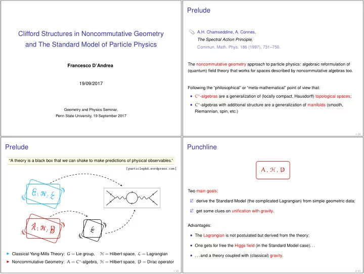19/09/2017 Following the “philosophical” or “meta-mathematical” point of view that: • C ∗ -algebras are a generalization of (locally compact, Hausdorff) topological spaces; • C ∗ -algebras with additional structure are a generalization of manifolds (smooth, Geometry and Physics Seminar, Riemannian, spin, etc.) Penn State University, 19 September 2017 1 / 21 Prelude Punchline “A theory is a black box that we can shake to make predictions of physical observables.” [ particlephd.wordpress.com ] A , H , D / G , H , L Two main goals: G , H , L � derive the Standard Model (the complicated Lagrangian) from simple geometric data; � � get some clues on unification with gravity. � A , H , D Advantages: A , H , D / L L / • The Lagrangian is not postulated but derived from the theory; • One gets for free the Higgs field (in the Standard Model case). . . ◮ Classical Yang-Mills Theory: G = Lie group, H = Hilbert space, L = Lagrangian • . . . and a theory coupled with (classical) gravity. ◮ Noncommutative Geometry: A = C ∗ -algebra, H = Hilbert space, D / = Dirac operator 1 / 21 2 / 21

The Lagrangian of the Standard Model Instructions: how to shake the red box L SM = − 1 ν − 1 µ − 1 1 µ − 1 2 ∂ ν g a µ ∂ ν g a µ − g s f abc ∂ µ g a ν g b µ g c 4 g 2 s f abc f ade g b µ g c ν g d µ g e ν − ∂ ν W + µ ∂ ν W − µ − M 2 W + µ W − 2 ∂ ν Z 0 µ ∂ ν Z 0 M 2 Z 0 µ Z 0 2 ∂ µ A ν ∂ µ A ν − igc w ( ∂ ν Z 0 µ ( W + µ W − ν − W + ν W − µ − µ ) 2 c 2 w µ )) − 1 Mathematical Physics Studies − Z 0 ν ( W + µ ∂ ν W − µ − W − µ ∂ ν W + µ ) + Z 0 µ ( W + ν ∂ ν W − µ − W − ν ∂ ν W + µ )) − igs w ( ∂ ν A µ ( W + µ W − ν − W + ν W − µ ) − A ν ( W + µ ∂ ν W − µ − W − µ ∂ ν W + µ ) + A µ ( W + ν ∂ ν W − µ − W − ν ∂ ν W + 2 g 2 W + µ W − µ W + ν W − ν + 1 ν ) − 1 2 g 2 W + µ W − ν W + µ W − ν + g 2 c 2 w ( Z 0 µ W + µ Z 0 ν W − ν − Z 0 µ Z 0 µ W + ν W − ν ) + g 2 s 2 w ( A µ W + µ A ν W − ν − A µ A µ W + ν W − ν ) + g 2 s w c w ( A µ Z 0 ν ( W + µ W − ν − W + ν W − µ ) − 2 A µ Z 0 µ W + ν W − 2 ∂ µ H∂ µ H − 2 M 2 α h H 2 − ∂ µ φ + ∂ µ φ − − 1 � 2 M 2 + 2 M g H + 1 � + 2 M 4 − 1 2 ∂ µ φ 0 ∂ µ φ 0 − β h 2 ( H 2 + φ 0 φ 0 + 2 φ + φ − ) H 3 + Hφ 0 φ 0 + 2 Hφ + φ − � H 4 + ( φ 0 ) 4 + 4 ( φ + φ − ) 2 g 2 α h − gα h M � 8 g 2 α h � g 2 Walter D. van Suijlekom µ H − 1 2 g M µ H − 1 + 1 + 4 ( φ 0 ) 2 φ + φ − + 4 H 2 φ + φ − + 2 ( φ 0 ) 2 H 2 � µ ( φ 0 ∂ µ φ − − φ − ∂ µ φ 0 ) − W − µ ( φ 0 ∂ µ φ + − φ + ∂ µ φ 0 ) µ ( H∂ µ φ − − φ − ∂ µ H ) − gMW + µ W − W + W + Z 0 µ Z 0 2 ig � � 2 g � c 2 w Noncommutative + 1 2 g 1 µ ( H∂ µ φ 0 − φ 0 ∂ µ H ) + M ( 1 µ ∂ µ φ + ) − igs 2 µ ( H∂ µ φ + − φ + ∂ µ H ) µ ∂ µ φ 0 + W + µ ∂ µ φ − + W − µ φ − − W − µ φ − − W − + W − � ( Z 0 Z 0 w MZ 0 µ ( W + µ φ + ) + igs w MA µ ( W + µ φ + ) c w c w c w Geometry and − ig 1 − 2 c 2 µ ( φ + ∂ µ φ − − φ − ∂ µ φ + ) + igs w A µ ( φ + ∂ µ φ − − φ − ∂ µ φ + ) − 1 − 1 8 g 2 1 H 2 + ( φ 0 ) 2 + 2 φ + φ − � H 2 + ( φ 0 ) 2 + 2 ( 2 s 2 w 4 g 2 W + µ W − w − 1 ) 2 φ + φ − � Z 0 � Z 0 µ Z 0 � µ µ 2 c w c 2 Particle Physics w − 1 2 g 2 s 2 µ φ + ) − 1 2 ig 2 s 2 µ φ + ) + 1 µ φ + ) + 1 µ φ + ) − g 2 s w µ φ − + W − µ φ − − W − µ φ − + W − µ φ − − W − w Z 0 µ φ 0 ( W + w Z 0 µ H ( W + 2 g 2 s w A µ φ 0 ( W + 2 ig 2 s w A µ H ( W + ( 2 c 2 w − 1 ) Z 0 µ A µ φ + φ − c w c w c w w A µ A µ φ + φ − + 1 � e λ γ µ e λ ) + 2 j ) − 1 � e ) e λ − ¯ ν ) ν λ − ¯ − g 2 s 2 2 ig s λ a q σ i γ µ q σ j ) g a e λ ( γ∂ + m λ ν λ ( γ∂ + m λ u λ j ( γ∂ + m λ u ) u λ j − ¯ d λ j ( γ∂ + m λ d ) d λ u λ j γ µ u λ 3 ( ¯ d λ j γ µ d λ ij ( ¯ µ − ¯ j + igs w A µ −( ¯ 3 ( ¯ j ) + ig j γ µ ( 4 j γ µ ( 1 − 8 j ) } + ig Z 0 ν λ γ µ ( 1 + γ 5 ) ν λ ) + ( ¯ e λ γ µ ( 4 s 2 w − 1 − γ 5 ) e λ ) + ( ¯ d λ 3 s 2 w − 1 − γ 5 ) d λ u λ 3 s 2 w + γ 5 ) u λ 2 W + � ν λ γ µ ( 1 + γ 5 ) U lep λκ e κ ) + ( ¯ u λ j γ µ ( 1 + γ 5 ) C λκ d κ � µ { ( ¯ j ) + ( ¯ √ ( ¯ j ) µ 4 c w 2 + ig ig ig � � 2 φ − � e κ U lep † κλ γ µ ( 1 + γ 5 ) ν λ ) + ( ¯ j C † e λ U lep † √ 2 W − ( ¯ d κ κλ γ µ ( 1 + γ 5 ) u λ j ) + √ 2 φ + � − m κ e ( ¯ ν λ U lep λκ ( 1 − γ 5 ) e κ ) + m λ ν ( ¯ ν λ U lep λκ ( 1 + γ 5 ) e κ � + √ m λ e ( ¯ λκ ( 1 + γ 5 ) ν κ ) µ 2 2 M 2 M m λ m λ m λ m λ − g ν λ ν λ ) − g e λ e λ ) + ig ν λ γ 5 ν λ ) − ig e λ γ 5 e λ ) − 1 ν κ − 1 e λ U lep † λκ ( 1 − γ 5 ) ν κ � − m κ ν e M φ 0 ( ¯ ν M φ 0 ( ¯ e ν λ M R ν λ M R ν ( ¯ M H ( ¯ M H ( ¯ 4 ¯ λκ ( 1 − γ 5 ) ˆ 4 ¯ λκ ( 1 − γ 5 ) ˆ ν κ 2 2 2 2 m λ m λ ig ig − g j ) − g 2 φ − � � 2 φ + � − m κ u λ j C λκ ( 1 − γ 5 ) d κ j ) + m λ u λ j C λκ ( 1 + γ 5 ) d κ � m λ d ( ¯ d λ j C † λκ ( 1 + γ 5 ) u κ j ) − m κ u ( ¯ d λ j C † λκ ( 1 − γ 5 ) u κ u u λ j u λ M H ( ¯ d d λ j d λ + √ d ( ¯ u ( ¯ + √ M H ( ¯ j ) j j 2 2 2 M 2 M + ig m λ j ) − ig m λ u M φ 0 ( ¯ M φ 0 ( ¯ u λ j γ 5 u λ d d λ j γ 5 d λ j ) 2 2 ( Chapter 12 → Phenomenology ) Lagrangian of the Standard Model with neutrino mixing and Majorana mass terms (Minkowski space, Feynman gauge fixing). M. Veltman, Diagrammatica: the path to Feynman diagrams , Cambridge Univ. Press, 1994. 3 / 21 4 / 21 Outline of the Talk Toolkit for Yang-Mills Theory Classical (i.e. before 2nd quantization) Euclidean gauge theory: Toolkit for Yang-Mills Theory 1 1 A complex Hilbert space H , typically: “Historical” background: 2 ψ v ◮ Grand Unified Theory (GUT) [ by Howard Georgi and Sheldon Glashow – 1974 ] ∈ ∈ L 2 ( M , E ) H = ⊗ V ◮ KK-theory [ Theodor K aluza – 1921, Oskar K lein – 1926 ] � �� �  sections of � ◮ Particle models and noncommutative geometry cpx vector bundle finite E → M dim. v.s. [ Alain Connes – 1996: “Gravity coupled with matter Usual QM interpretation: ψ = probability amplitude; and foundation of non-commutative geometry”, v = internal degrees of freedom (spin, charge, etc.) with John Lott – 1991, with Ali Chamseddine – since 1996 ] Remark: in the Standard Model, rk ( E ) = 4 (spinor bundle on a 4 -dim. manifold). The spin degree of freedom is counted twice (in E and in V ), cf. fermion doubling : Clifford Structures in Noncommutative Geometry and Morita Equivalence 3 F . Lizzi, G. Mangano, G. Miele, G. Sparano, Phys. Rev. D 55 (1997), 6357–6366. [ joint with Ludwik Dabrowski and Andrzej Sitarz ] Another doubling is typical of Euclidean field theories and is cured after Wick rotation, cf. F . D’Andrea, M. Kurkov and F . Lizzi, Phys. Rev. D 94, 025030 (2016). 5 / 21 6 / 21