Propagating Error Backward Hyperparameters for Neural Networks } - - PowerPoint PPT Presentation

SLIDE 1

1

Class #18: Back-Propagation; Tuning Hyper-Parameters

Machine Learning (COMP 135): M. Allen, 04 Nov. 19

1

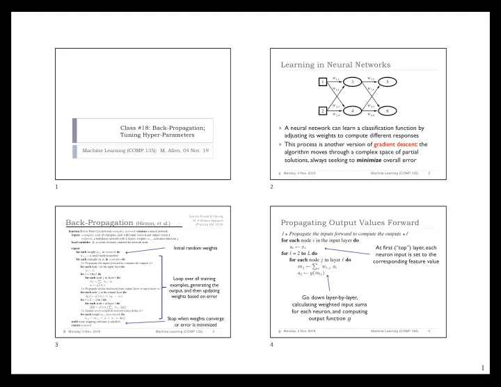
Learning in Neural Networks

} A neural network can learn a classification function by

adjusting its weights to compute different responses

} This process is another version of gradient descent: the

algorithm moves through a complex space of partial solutions, always seeking to minimize overall error

Monday, 4 Nov. 2019 Machine Learning (COMP 135) 2

w3,5

3,6

w

4,5

w

4,6

w 5 6 w1,3

1,4

w

2,3

w

2,4

w 1 2 3 4

2

function BACK-PROP-LEARNING(examples, network) returns a neural network inputs: examples, a set of examples, each with input vector x and output vector y network, a multilayer network with L layers, weights wi,j, activation function g local variables: ∆, a vector of errors, indexed by network node repeat for each weight wi,j in network do wi,j ← a small random number for each example (x, y) in examples do /* Propagate the inputs forward to compute the outputs */ for each node i in the input layer do ai ← xi for ℓ = 2 to L do for each node j in layer ℓ do inj ← P

i wi,j ai

aj ← g(inj) /* Propagate deltas backward from output layer to input layer */ for each node j in the output layer do ∆[j] ← g′(inj) × (yj − aj) for ℓ = L − 1 to 1 do for each node i in layer ℓ do ∆[i] ← g′(ini) P

j wi,j ∆[j]

/* Update every weight in network using deltas */ for each weight wi,j in network do wi,j ← wi,j + α × ai × ∆[j] until some stopping criterion is satisfied return network

Back-Propagation (Hinton, et al.)

Monday, 4 Nov. 2019 Machine Learning (COMP 135) 3

Initial random weights Loop over all training examples, generating the

• utput, and then updating

weights based on error Stop when weights converge

• r error is minimized

Source: Russel & Norvig, AI: A Modern Approach (Prentice Hal, 2010)

3

for each example x y in do /* Propagate the inputs forward to compute the outputs */ for each node i in the input layer do ai ← xi for ℓ = 2 to L do for each node j in layer ℓ do inj ← P

i wi,j ai

aj ← g(inj) /* Propagate deltas backward from output layer to input laye

Propagating Output Values Forward

Monday, 4 Nov. 2019 Machine Learning (COMP 135) 4

At first (“top”) layer, each neuron input is set to the corresponding feature value Go down layer-by-layer, calculating weighted input sums for each neuron, and computing

• utput function g

4

SLIDE 2

2

/* Propagate deltas backward from output layer to input layer */ for each node j in the output layer do ∆[j] ← g′(inj) × (yj − aj) for ℓ = L − 1 to 1 do for each node i in layer ℓ do ∆[i] ← g′(ini) P

j wi,j ∆[j]

/* Update every weight in network using deltas */ for each weight wi,j in network do wi,j ← wi,j + α × ai × ∆[j] until some stopping criterion is satisfied

Propagating Error Backward

Monday, 4 Nov. 2019 Machine Learning (COMP 135) 5

At output (“bottom”) layer, each delta-value is set to the error on that neuron, multiplied by the derivative of function g Go bottom-up and set delta to derivative value multiplied by sum of deltas at the next layer down (weighting each such value appropriately) After all the delta values are computed, update weights on every node in the network

5

Hyperparameters for Neural Networks

} Multi-layer (deep) neural networks involve a number of

different possible design choices, each of which can affect classifier accuracy:

} Number of hidden layers } Size of each hidden layer } Activation function employed } Regularization term (controls over-fitting)

} This is not unique to neural networks

} Logistic regression: regularization (C parameter in sklearn), class

weights, etc.

} SVM: kernel type, kernel parameters (like polynomial degree), error

penalty (C again), etc.

} Question is often how we can tune these model control

parameters effectively to find best combinations

Monday, 4 Nov. 2019 Machine Learning (COMP 135) 6

6

Heldout Cross-Validation

} We can use k-fold cross-validation techniques to estimate the

real effectiveness of various parameter settings:

1.

Divide labeled data into k folds, each of size 1/k

2.

Repeat k times:

a.

Hold aside one of the folds; train on the remaining (k – 1); test on the heldout data

b.

Record classification error for both training and heldout data

3.

Average over the k trials

} This can give us a more robust estimate of real effectiveness } It can also allow us to better detect over-fitting: when average

heldout error is significantly worse than average training error, model has grown too complex or otherwise problematic

Monday, 4 Nov. 2019 Machine Learning (COMP 135) 7

7

Modifying Model Parameters

} Using heldout validation techniques, we can begin to

explore various parts of the hyperparameter-space

} In each case, we try to maximize average performance on the

heldout validation data

} For example: number of layers in a neural network can

be explored iteratively, starting with one layer, and increasing one at a time (up to some reasonable) limit until over-fitting is detected

} Similarly, we can explore a range of layer sizes, starting

with hidden layers of size equal to the number of input features, and increasing in some logarithmic manner until

• ver-fitting occurs, or some practical limits reach

Monday, 4 Nov. 2019 Machine Learning (COMP 135) 8

8

SLIDE 3

3 Using Grid Search for Tuning

} One basic technique is to list out the different values of

each parameter that we want to test, and systematically try different combinations of those values

} For P distinct tuning parameters, defines a P-dimensional space

(or “grid”), that we can explore, one combination at a time

} In many cases, since building, training, and testing the

models for each combination all take some time, we may find that there are far too many such combinations to try

} One possibility: many such models can be explored in parallel,

allowing large numbers of combinations to be compared at the same time, given sufficient resources

Monday, 4 Nov. 2019 Machine Learning (COMP 135) 9

9

Costs of Grid Search

} When we have large numbers of combinations of possible

parameters, we may decide to limit the range of some of the parts of our “grid” for feasibility

} For example, we might try:

1.

# Hidden layers: 1, 2, …, 10

2.

Layer size: N, 2N, 5N, 10N, 20N (N: # input features)

3.

Activation: Sigmoid, ReLU, tanh

4.

Regularization (alpha): 10-5, 10-3, 10-1, 101, 103

} Produces (10 x 5 x 3 x 5) = 750 different models

} If we are doing 10-fold validation, need to run 7,500 total tests } Still only a small fragment of the possible parameter-space

Monday, 4 Nov. 2019 Machine Learning (COMP 135) 10

10

Random Search

} Instead of limiting our grid even further, or trying to spend

even more time on more combinations, we might try to randomize the process

} Instead of limiting values, we choose randomly from any of a

(larger) range of values:

1.

# Hidden layers: [1, 20]

2.

Layer size: [8, 1024]

3.

Activation: [Sigmoid, ReLU, tanh]

4.

Regularization (alpha): [10-7,107]

} For each of these, we assign a probability distribution over its

values (uniform or otherwise)

} We may presume these distributions are independent of one another

} For T tests, we sample each of the ranges for one possible

value, giving us T different combinations of those values

Monday, 4 Nov. 2019 Machine Learning (COMP 135) 11

11

Performance of Random Search

}

This technique can sometimes out-perform grid search

}

When using a grid, it is sometimes possible that we just miss some intermediate, and important, value completely

}

The random approach can often hit upon the better combinations with the same (or far less) testing involved

Monday, 4 Nov. 2019 Machine Learning (COMP 135) 12 Grid Layout Random Layout

Unimportant parameter Important parameter Unimportant parameter Important parameter

e 1: Grid and random search of nine trials for optimizing a function f(x,y) = g(x) + h(y) ≈ g(x) with low effective dimensionality. Above each square g(x) is shown in green, and left of each square h(y) is shown in yellow. With grid search, nine trials only test g(x) in three distinct places. With random search, all nine trials explore distinct values of

• g. This failure of grid search is the rule rather than the exception in high dimensional

hyper-parameter optimization. From: J. Bergstra & Y. Bengio, “Random search for hyper- parameter optimization,” Journal of Machine Learning Research 13 (2012).

12

SLIDE 4

4

Performance of Random Search

Monday, 4 Nov. 2019 Machine Learning (COMP 135) 13 From: J. Bergstra & Y. Bengio, “Random search for hyper- parameter optimization,” Journal of Machine Learning Research 13 (2012). 1 2 4 8 16 32

experiment size (# trials)

0.3 0.4 0.5 0.6 0.7 0.8 0.9 1.0

accuracy mnist rotated

Performance for grid search over 100 different neural network parameter combinations Statistically significant improvement for as few as 8 randomly chosen combination models

13

This Week

} T

• pics: Neural Networks

} Project 01: due Monday, 04 November, 4:15 PM

} Can be handed in without penalty untilWed., 06 Nov., 4:15 PM

} Homework 04: due Wednesday, 06 November, 9:00 AM } Office Hours: 237 Halligan, Tuesday, 11:00 AM – 1:00 PM

} TA hours can be found on class website as well

Monday, 4 Nov. 2019 Machine Learning (COMP 135) 14

14