Program Efficiency CSE 1030 The cost of executing a program or - PowerPoint PPT Presentation

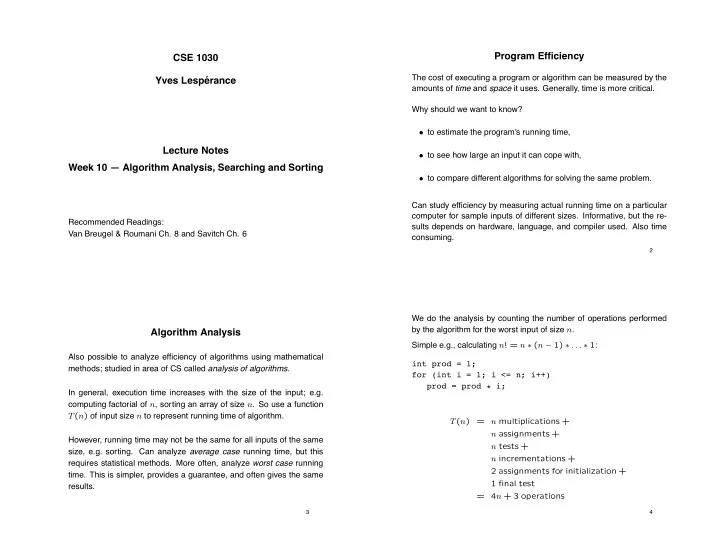
Program Efficiency CSE 1030 The cost of executing a program or algorithm can be measured by the Yves Lesp´ erance amounts of time and space it uses. Generally, time is more critical. Why should we want to know? • to estimate the program’s running time, Lecture Notes • to see how large an input it can cope with, Week 10 — Algorithm Analysis, Searching and Sorting • to compare different algorithms for solving the same problem. Can study efficiency by measuring actual running time on a particular computer for sample inputs of different sizes. Informative, but the re- Recommended Readings: sults depends on hardware, language, and compiler used. Also time Van Breugel & Roumani Ch. 8 and Savitch Ch. 6 consuming. 2 We do the analysis by counting the number of operations performed by the algorithm for the worst input of size n . Algorithm Analysis Simple e.g., calculating n ! = n ∗ ( n − 1) ∗ . . . ∗ 1 : Also possible to analyze efficiency of algorithms using mathematical int prod = 1; methods; studied in area of CS called analysis of algorithms . for (int i = 1; i <= n; i++) prod = prod * i; In general, execution time increases with the size of the input; e.g. computing factorial of n , sorting an array of size n . So use a function T ( n ) of input size n to represent running time of algorithm. T ( n ) = n multiplications + n assignments + However, running time may not be the same for all inputs of the same n tests + size, e.g. sorting. Can analyze average case running time, but this n incrementations + requires statistical methods. More often, analyze worst case running 2 assignments for initialization + time. This is simpler, provides a guarantee, and often gives the same 1 final test results. = 4 n + 3 operations 3 4

Approximating, we drop the lower order term 3 as it becomes neglige- Sorting able when n gets large. Also, we drop the constant 4 since the time to perform an operation depends on the computer. So we say that T ( n ) Sorting an array or list is a very common operation. The array/list is is O ( n ) , i.e. Big-Oh n . sorted if all its elements appear in the right order. Big-oh can be defined formally: What “right order” means is application dependent. E.g. sort array of Student objects so that they appear in increasing order of student f ( n ) is O ( g ( n )) iff there exist positive constants C and K such that number. Could also sort by names using lexicographic order. Another f ( n ) ≤ C · g ( n ) for all n ≥ K . e.g.: could sort marks in a class in decreasing order. Big-oh gives us an estimate of how fast running time grows as n grows. It is much easier to find an item if the array/list is sorted than if it is not (e.g. in a phone book). In doing the analysis, don’t need to count all operations, only pick one that reflects the overall performance of the algorithm — is executed There are many different algorithms for array sorting. Much work has most often, is in the inner most loop. E.g. for iterative factorial, count been done to analyse them and determine which are the best in terms multiplications. E.g. for sorting: count array accesses or comparisons of running time. between elements. 5 6 Merge Sort — A Recursive Array Sorting Algorithm Steps: public static void merge(int[] a, int from, int mid, int to) { // create temporary array 1. divide the array into 2 halves; int both = to - from + 1; int[] tempA = new int[both]; 2. sort each half recursively; // merge until one array runs out int i1 = from; int i2 = mid + 1; 3. merge the sorted halves back into a single array. int j = 0; while(i1 <= mid && i2 <= to) { if (a[i1] < a[i2]) public static void mergeSort(int[] a, int from, int to) { tempA[j] = a[i1]; { if(from == to) return; i1++; int mid = (from + to) / 2; } // sort both halves recursively and merge back else mergeSort(a, from, mid); { tempA[j] = a[i2]; mergeSort(a, mid + 1, to); i2++; merge(a, from, mid, to); } } j++; } public static void sort(int[] a) { mergeSort(a, 0, a.length - 1); } 7 8

Tracing execution of Merge Sort on a = [ 18, 33, 4, 21, 17, 35, 20 ] mergeSort(a,0, 6) calls mergeSort(a,0,3) mergeSort(a,0,3) calls mergeSort(a,0,1) // copy rest of remaining half mergeSort(a,0,1) calls mergeSort(a,0,0) while(i1 <= mid){ mergeSort(a,0,0) returns tempA[j] = a[i1]; mergeSort(a,0,1) calls mergeSort(a,1,1) i1++; mergeSort(a,1,1) returns j++; mergeSort(a,0,1) calls merge(a,0,0,1) } merge(a,0,0,1) merges [18] and [33] returns with a unchanged while(i2 <= to){ mergeSort(a,0,1) returns with a unchanged tempA[j] = a[i2]; mergeSort(a,0,3) calls mergeSort(a,2,3) i2++; mergeSort(a,2,3) calls mergeSort(a,2,2) j++; mergeSort(a,2,2) returns } mergeSort(a,2,3) calls mergeSort(a,3,3) // copy tempA back into a mergeSort(a,3,3) returns for (j = 0; j < both; j++) mergeSort(a,2,3) calls merge(a,2,2,3) a[from + j] = tempA[j]; merge(a,2,2,3) merges [4] and [21] returns with a unchanged } mergeSort(a,2,3) returns with a unchanged mergeSort(a,0,3) calls merge(a,0,1,3) merge(a,0,1,3) merges [18, 33] and [4, 21] returns with a = [4, 18, 21, 33, 17, 35, 20] mergeSort(a,0,3) returns with a as above 9 10 Proof by Induction of Correctness and Termination for Merge Sort mergeSort(a,0,6) calls mergeSort(a,4,6) mergeSort(a,4,6) calls mergeSort(a,4,5) mergeSort(a,4,5) calls mergeSort(a,4,4) Let’s assume that merge(a,i,m,j) is correct and terminates, i.e. mergeSort(a,4,4) returns merges sorted sub-arrays a[i..m] and a[m+1..j] into a single sorted mergeSort(a,4,5) calls mergeSort(a,5,5) mergeSort(a,5,5) returns sub-array a[i..j] . This can be proven using loop invariants. mergeSort(a,4,5) calls merge(a,4,4,5) merge(a,4,4,5) merges [17] and [35] returns with a unchanged mergeSort(a,4,5) returns with a unchanged We prove correctness and termination of the mergeSort(a,i,j) mergeSort(a,4,6) calls mergeSort(a,6,6) method by induction on the size n of the sub-array considered, i.e. mergeSort(a,6,6) returns mergeSort(a,4,6) calls merge(a,4,5,6) n = j − ( i − 1) . merge(a,4,5,5) merges [17, 35] and [20] returns with a = [4, 18, 21, 33, 17, 20, 35] mergeSort(a,4,6) returns with a as above 1) Base case n = 1 : then mergeSort(a,i,j) immediately returns, mergeSort(a,0,6) calls merge(a,0,3,6) and a subarray of size 1 is always sorted. So the method is correct. merge(a,0,3,6) merges [4, 18, 21, 33] and [17, 20, 35] returns with a = [4, 17, 18, 20, 21, 33, 35] mergeSort(a,0,6) returns with a as above 2) For the recursive case: Assume that mergeSort(a,i,j) is correct and terminates for all sizes n ≤ k (induction hypothesis). 11 12

We must prove that that the method is correct for size n = k + 1 . Analysis of Running Time of Merge Sort Then mergeSort(a,i,j) calls mergeSort(a,i,mid) and mergeSort(a,mid+1,j) . In both cases, the size of the sub-array Merging 2 arrays containing a total of n elements requires n − 1 com- involved is ≤ k , so by the induction hypothesis these two calls correctly parisons in the worst case (when neither half runs out early). If you sort the sub-arrays a[i..mid] and a[mid+1..j] . want to count all operations, then the running time will be C 1 n + C 2 where C 1 and C 2 are constants. If you drop the lower order term, you After the recursive call, merge(a,i,mid,j) is called to merge the get C 1 n . two sorted sub-arrays. By our assumption that merge is correct, this results in a[i,j] being sorted. The running time for the complete sorting of an array of size n can be specified as a recurrence relation: So mergeSort is correct for size n = k + 1 . � C 2 if n ≤ 1 T ( n ) = 2 T ( n/ 2) + C 1 n otherwise Thus for all natural numbers n mergeSort(a,i,j) correctly sorts the sub-array a[i..j] where n is the size of the sub-array and termi- nates. 13 14 Suppose that n is a power of 2, i.e. n = 2 m . Then we can keep applying the relation until n reaches 2 0 = 1 : 2 m T ( n/ 2 m ) + mC 1 n T ( n ) = C 2 2 m + C 1 mn since T ( n/ 2 m ) = T (1) = C 2 = = C 2 n + C 1 n log 2 n since m = log 2 n There are general methods for solving recurrence relations, but let’s do = O ( n log n ) it from first principles. If n/ 2 > 1 , we can apply the recurrence relation to T ( n/ 2) to get: Thus, the running time of merge sort grows much more slowly than T ( n ) = 2(2 T ( n/ 4) + C 1 n/ 2) + C 1 n that of many other sorting algorithms whose running time is O ( n 2 ) , = 4 T ( n/ 4) + 2 C 1 n e.g. selection sort, insertion sort, etc.: n 2 n n log e n 10 23 100 100 460 10 , 000 10 3 6 . 9 10 3 10 6 10 6 13 . 8 10 6 10 12 15 16