Profile-Guided Optimizations Last time Instruction scheduling - PDF document

Profile-Guided Optimizations Last time – Instruction scheduling – Register renaming – Balanced Load Scheduling – Loop unrolling – Software pipelining Today – More instruction scheduling – Profiling – Trace scheduling CS553 Lecture Profile-Guided Optimizations 2 Motivation for Profiling Limitations of static analysis – Compilers can analyze possible paths but must behave conservatively – Frequency information cannot be obtained through static analysis 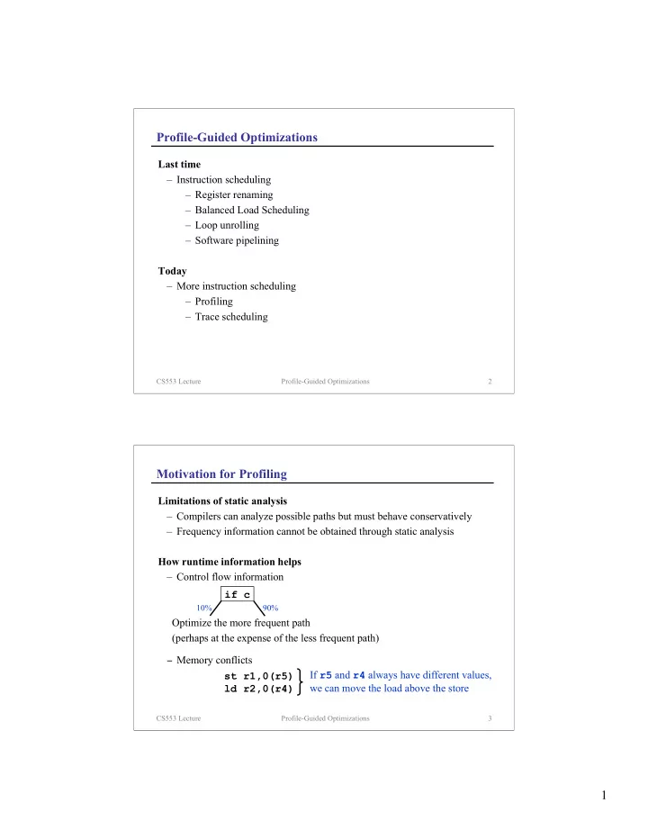How runtime information helps – Control flow information if c 10% 90% Optimize the more frequent path (perhaps at the expense of the less frequent path) − Memory conflicts If r5 and r4 always have different values, st r1,0(r5) ld r2,0(r4) we can move the load above the store CS553 Lecture Profile-Guided Optimizations 3 1

Profile-Guided Optimizations Basic idea – Instrument and run program on sample inputs to get likely runtime behavior – Can use this information to improve instruction scheduling – Many other uses – Code placement – Inlining – Value speculation – Branch prediction – Class-based optimization (static method lookup) CS553 Lecture Profile-Guided Optimizations 4 Profiling Issues Profile data – Collected over whole program run – May not be useful (unbiased branches) – May not reflect all runs – May be expensive and inconvenient to gather – Continuous profiling [Anderson 97] – May interfere with program CS553 Lecture Profile-Guided Optimizations 5 2

Control-Flow Profiles Commonly gather two types of information – Execution frequencies of basic blocks – Branch frequencies of conditional branches – Represent information in a weighted flow graph execution frequencies 1 100 2 100 branch frequencies 30 70 3 4 70 30 Instrumentation – Insert instrumentation code at basic block entrances and before each branch – Take average of values from multiple training runs – Fairly inexpensive CS553 Lecture Profile-Guided Optimizations 6 Code Motion Using Control Flow Profiles Code motion across basic blocks – Increased scheduling freedom A B − If we want to move s1 to A, we must move C s1 s1 to both A and B move code above a join s1 A − If we want to move s1 to B, we must B C move s1 to both B and C move code below a split CS553 Lecture Profile-Guided Optimizations 7 3

Code Motion Using Control Flow Profiles (cont) Code motion across basic blocks – Increased scheduling freedom A s1 B A B s1 C C ′ C move code below a join tail duplication prevents B → C from seeing s1 − If we want to move s1 from B to A and if s1 A would destroy a value along the A → C path, B s1 C do renaming (in hardware or software) move code above a split − What if s1 might cause an exception? CS553 Lecture Profile-Guided Optimizations 8 Memory-Dependence Profiles Gather information about memory conflicts – Frequencies of address matches between pairs of loads and stores – Attempts to answer the question: Are two references independent of one another? – Concentrate on ambiguous reference pairs (those that the compiler cannot figure out) st1: store r5 (st1, ld2, 7) If this number is low, we can ld2: load r4 speculatively assume that st1 and ld2 do not conflict Instrumentation – Much more expensive (in both space and time) to gather than control flow information – First perform control flow profiling – Apply only to most frequently executed blocks CS553 Lecture Profile-Guided Optimizations 9 4

Trace Scheduling [Fisher 81] and [Ellis 85] Basic idea – We want large blocks to create large scheduling windows, but basic blocks are small because branches are frequent – Create superblocks to increase scheduling window – Use profile information to create good superblocks – Optimize each superblock independently Superblocks – A sequence of basic blocks with a single entrance and multiple exits 1 Goals a superblock – Want large superblocks 2 – Want to avoid early exits – Want blocks that match actual execution paths 3 4 CS553 Lecture Profile-Guided Optimizations 10 Trace Scheduling (example) trace: b[i] = “old” b[i] = “old” a[i] = ... a[i] = ... if (a[i]>0) then b[i]=“new”; b[i]=“new”; c[i] = ... else if (a[i]<=0) then goto repair stmt X continue: stmt Y ... endif c[i] = ... repair: restore old b[i] stmt X stmt Y recalculate c[i]? goto continue CS553 Lecture Profile-Guided Optimizations 11 5

Trace Scheduling (cont) Three steps 1. Create superblocks 2. Enlarge superblocks 3. Compact (optimize) superblocks 1. Superblock formation − Create traces using mutual-most-likely heuristic (two blocks A and B are mutual-most-likely if B is the most likely successor of A, and A is the most likely predecessor of B) D A − A trace is a maximal sequence of mutual- 30 10 70 most-likely blocks that does not contain a back B C edge 70 10 − Each block belongs to exactly one trace E CS553 Lecture Profile-Guided Optimizations 12 Trace Scheduling (cont) 1. Superblock formation (cont) – Convert traces into Superblocks – Use tail duplication to eliminate side entrances A A 70 30 70 30 trace superblock B C B C 70 10 70 10 E ′ E E − Tail duplication increases code size CS553 Lecture Profile-Guided Optimizations 13 6

Trace Scheduling (cont) 2. Superblock enlargement – Enlarge superblocks that are too small – Code expansion can hurt i-cache performance Three techniques for enlargement – Branch target expansion – If the last branch in a superblock is likely to jump to the start of another superblock, append the contents of the target superblock to the first superblock – Loop peeling – Loop unrolling – These last two techniques apply to superblock loops, which are superblocks whose last blocks are likely to jump to their first blocks – Assume that each loop body has a single dominant path CS553 Lecture Profile-Guided Optimizations 14 Trace Scheduling (cont) 3. Optimizations – Perform list scheduling for each superblock – Memory-dependence profiles can be used to speculatively assume that load/store pairs do not conflict – Insert repair code in case the assumption is incorrect – Software pipelining CS553 Lecture Profile-Guided Optimizations 15 7

Speculation based on memory-dependence profiles (example) trace: b[i] = “old” b[i] = “old” a[i] = ... c[i] = a[j] if (a[i]>0) then a[i] = ... b[i]=“new”; b[i]=“new”; else if (i==j) then goto deprepair stmt X if (a[i]<=0) then goto repair stmt Y continue: endif ... c[i] = a[j] deprepair: c[i] = a[i] if (a[i]<=0) then goto repair goto continue repair: restore old b[i] stmt X stmt Y goto continue CS553 Lecture Profile-Guided Optimizations 16 Enhancements to Profile-Guided Code Scheduling Path profiling [Ball and Larus 96] – Collect information about entire paths instead of about individual edges 50 50 50 50 50 50 50 50 50 50 50 50 Path profiles Path profiles Edge profiles – Limit paths to some specified length (can thus handle loops) – Can also stop paths at back edges – Disadvantages of path profiling? CS553 Lecture Profile-Guided Optimizations 17 8

Lessons Larger scope helps – How can we increase scope? How do we schedule across control dependences? Static information is limited – Use profiles – How else can profiles be used in optimization? – Can we do these kinds of optimizations at runtime? CS553 Lecture Profile-Guided Optimizations 18 Concepts Instruction scheduling – Software pipelining – Trace scheduling – Both use profile information – Both look at scopes beyond basic blocks Miscellany – Path profiling – Speculative hedging CS553 Lecture Profile-Guided Optimizations 19 9

Next Time Reading – Mahlke’92 Lecture – Speculation and predication CS553 Lecture Profile-Guided Optimizations 20 10