Probability Basics Probabilistic Inference Martin Emms October 1, - PowerPoint PPT Presentation

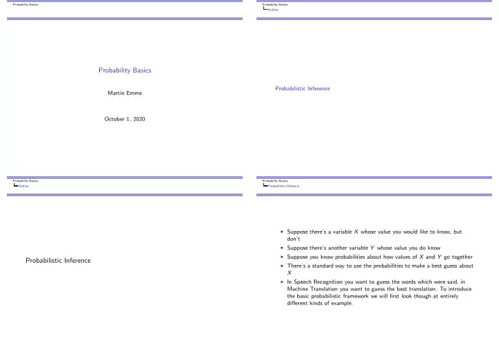
Probability Basics Probability Basics Outline Probability Basics Probabilistic Inference Martin Emms October 1, 2020 Probability Basics Probability Basics Outline Probabilistic Inference ◮ Suppose there’s a variable X whose value you would like to know, but don’t ◮ Suppose there’s another variable Y whose value you do know ◮ Suppose you know probabilities about how values of X and Y go together Probabilistic Inference ◮ There’s a standard way to use the probabilities to make a best guess about X ◮ In Speech Recognition you want to guess the words which were said, in Machine Translation you want to guess the best translation. To introduce the basic probabilistic framework we will first look though at entirely different kinds of example.

Probability Basics Duda and Hart’s fish example Probabilistic Inference Suppose there are 2 types of fish. You might want to design a fish-sorter which seeks to distinguish between the 2 types of fish (eg. salmon vs. sea bass) by the value of some observable attribute, possibly an attribute a camera can easily measure (eg. lightness of skin) Can be formalised by representing a fish with 2 variables ◮ ω : a variable for the type of fish (values ω 1 , ω 2 ) ◮ x : observed skin brightness images from Duda and Hart, Pattern Recognition Then suppose these distributions are known: 1. P ( ω ) 2. P ( x | ω ) ( Jargon : P ( x | ω ) might be called the class conditional probability ) If you observe a fish with a particular value for x, what is the best way to use the observation to predict its category? Probability Basics Probability Basics Probabilistic Inference Probabilistic Inference Maximise Joint Probability Maximise Conditional Probability The following seems (and is) sensible An equally sensible and in fact equivalent intuition for how to pick ω is to maximise conditional probability of ω given x ie. choose arg max P ( ω, x ) ω choose arg max P ( ω | x ) ω i.e. pick the value for ω which together with x gives the likeliest pairing. Using the product rule this can be recast as i.e. pick the value for ω which is likeliest given x . This turns out to give exactly the same criterion as the maximise-joint before in (1), as follows ’Bayesian Classifier’ arg max P ( ω | x ) = arg max P ( ω, x ) / P ( x ) (2) choose arg max P ( x | ω ) P ( ω ) (1) ω ω ω = arg max P ( x | ω ) P ( ω ) / P ( x ) (3) ω = arg max P ( x | ω ) P ( ω ) (4) So if you know both P ( x | ω ) and P ( ω ) for the two classes ω 1 and ω 2 can now ω pick the one which maximises P ( x | ω ) P ( ω ) (2) is by definition of conditional probablility, (3) is by Product Rule, and (4) though widely given the name ’Bayesian Classifier’ this really doing nothing because denominator P ( x ) does not mention ω , it does not vary with ω and more than saying pick the ω which makes the combination you are looking at can be left out as likely as possible.

Probability Basics Probabilistic Inference The following shows hypothetical plots of P ( x | ω 1 ) and P ( x | ω 2 ) images from Duda and Hart, Pattern Recognition Assuming a priori probs P ( ω 1 ) = 2 / 3, P ( ω 2 ) = 1 / 3, the plots below show P ( ω 1 , x ) and P ( ω 2 , x ), normalised at each x by P ( x ) (ie. it shows P ( ω | x )) images from Duda and Hart, Pattern Recognition ◮ Basically up to about x = 12 . 5, P ( x | ω 2 ) > P ( x | ω 1 ) and thereafter the relation is the other way around. ◮ but this does not mean ω 2 should be chosen for x < 12 . 5, and ω 1 otherwise. ◮ the plot shows only half of the P ( x | ω ) P ( ω ) referred to in the decision function (1): the other factor is the a priori likelihood P ( ω ) ◮ So roughly for x < 10 or 11 < x < 12, ω 2 is the best-guess ◮ So roughly for 10 < x < 11 or 12 < x , ω 1 is the best-guess Probability Basics Probability Basics Probabilistic Inference Probabilistic Inference Optimality ’prior’ and ’posterior’ ◮ have seen that this Bayesian recipe is guaranteed to give the least error in the long term: if arg max P ( ω | x ) = arg max ( p ( x | ω ) p ( ω )) you know the probs p ( x | ω ) and p ( ω ), you cannot do better than always ω ω guessing arg max ω ( p ( x | ω ) p ( ω )) ◮ often p ( ω ) is termed the prior probability (guessing the fish before looking) there’s some special cases ◮ often p ( ω | x ) is termed the posterior probability (guessing the fish after ◮ if p ( x | ω 1 ) = p ( x | ω 2 ), the evidence tells you nothing, and the decision rests looking) entirely on p ( ω 1 ) vs p ( ω 2 ) ◮ if p ( ω 1 ) = p ( ω 2 ), then the decision rests entirely on the class-conditionals: arg max P ( ω | x ) = arg max ( p ( x | ω ) p ( ω ) ) p ( x | ω 1 ) vs. p ( x | ω 2 ) � �� � ���� ω ω posterior prior

Probability Basics Probability Basics Probabilistic Inference Probabilistic Inference Jedward example A sound-bite may or may not have been produced by JedWard. A ◮ So can choose by considering P ( x | ω ) P ( ω ). sound-bite may or may not contain the word OMG . ◮ it can sometimes surprise that for all the ω , P ( x | ω ) P ( ω ) might be tiny You hear OMG and want to work out the probability that the speaker and not sum to one: but recall its a joint probability, so it incorporates is Jedward the probability of the evidence, which might not be very likely. Formalize with 2 discrete variables ◮ It also must be the case that ◮ discrete Speaker , values in { Jedward , Other } � � P ( x ) = P ( ω, x ) = P ( x | ω ) P ( ω ) ◮ discrete OMG , values in { true , false } ω ω Let jed stand for Speaker = Jedward , omg stand for OMG = true so P ( x ) can be obtained by summing P ( x | ω ) P ( ω ) for the different values Then suppose these individual probabilities are known of ω , the same term whose maximum value is searched for in (1) 1. p ( jed ) = 0 . 01 ◮ so to get the true conditional p ( ω | x ), can get the two P ( x | ω 1 ) P ( ω 1 ) and 2. p ( omg | jed ) = 1 . 0 P ( x | ω 2 ) P ( ω 2 ) values and then divide each by their sum 3. p ( omg |¬ jed ) = 0 . 1 ◮ Without dividing through by P ( x ) you get basically the much smaller joint choosing by Bayesian rule (1) probabilities. The maximum occurs for the same ω as the conditional probability and the ratios amongst them are the same as amongst the p ( omg | jed ) p ( jed ) = 0 . 01 , p ( omg |¬ jed ) p ( ¬ jed ) = 0 . 099 conditional probs. hence choose ¬ jed Probability Basics Probability Basics Probabilistic Inference Probabilistic Inference if want real probability p ( jed | omg ) summing these alternatives and normalising by this (effectively dividing by p ( omg )) gives p ( jed | omg ) = 0 . 0917 , p ( ¬ jed | omg ) = 0 . 9083 we have The posterior probability of p ( jed | omg ) is quite small, even though p ( omg | jed ) p ( omg | jed ) p ( jed ) = 0 . 01 , p ( omg |¬ jed ) p ( ¬ jed ) = 0 . 099 is large. This is due to the quite low prior p ( jed ), and non negligible p ( omg |¬ jed ) = 0 . 1 both values are quite small, and they do not sum to 1 Raising the prior prob for jed to p ( jed ) = 0 . 1, changes the outcome to this is because they are alternate expressions for the joint probabilities p ( jed | omg ) = 0 . 526 , p ( ¬ jed | omg ) = 0 . 474 p ( omg , jed ) and p ( omg , ¬ jed ), and summing these gives the total omg probability, which is not that large. Or alternatively decreasing the prob of hearing OMG from anyone else to 0 . 001, changes the outcome to p ( jed | omg ) = 0 . 917 , p ( ¬ jed | omg ) = 0 . 083

Probability Basics Probability Basics Probabilistic Inference Probabilistic Inference Recap Further reading Joint Probability P ( X , Y ) Marginal Probability P ( X ) = � Y P ( X , Y ) Conditional Probability P ( Y | X ) = P ( X , Y ) . . . really count ( X , Y ) P ( X ) count ( X ) see the course pages under ’Course Outline’ for details on particular parts of of Product Rule P ( X , Y ) = P ( Y | X ) × P ( X ) particular books which can serve as further sources of information concerning the topics introduced by the preceding slides Chain Rule P ( X , Y , Z ) = p ( Z | ( X , Y )) × P ( X , Y ) = p ( Z | ( X , Y )) × P ( Y | X ) × p ( X ) Conditional Independence P ( X | Y , Z ) = P ( X | Z ) ie. X ignores Y given Z Bayesian Inversion P ( X | Y ) = P ( Y | X ) P ( X ) P ( Y ) Inference to infer X from Y choose X = arg max X P ( Y | X ) P ( X )