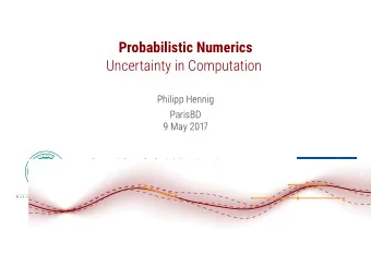
Probabilistic Numerics Part I Integration and Differential - PowerPoint PPT Presentation

Probabilistic Numerics – Part I – Integration and Differential Equations Philipp Hennig MLSS 2015 18 / 07 / 2015 Emmy Noether Group on Probabilistic Numerics Department of Empirical Inference Max Planck Institute for Intelligent Systems Tübingen, Germany

Information Content of Partial Computations division with remainder ÷ = 2 3 7 3 6 7 3 6 X X . X X 1 ,

Information Content of Partial Computations division with remainder ÷ = 2 3 7 3 6 7 3 6 3 X . X X 2 2 0 8 0 1 6 5 6 1 ,

Information Content of Partial Computations division with remainder ÷ = 2 3 7 3 6 7 3 6 3 2 . X X 2 2 0 8 0 1 6 5 6 1 4 7 2 1 8 4 1 ,

Information Content of Partial Computations division with remainder ÷ = 2 3 7 3 6 7 3 6 3 2 2 . X 2 2 0 8 0 1 6 5 6 1 4 7 2 1 8 4 1 4 7 2 . 3 6 8 . 1 ,

Information Content of Partial Computations division with remainder ÷ = 2 3 7 3 6 7 3 6 3 2 2 5 . 2 2 0 8 0 1 6 5 6 1 4 7 2 1 8 4 1 4 7 2 . 3 6 8 . 3 6 . 8 0 1 ,

What about ML computations? Contemporary computational tasks are more challenging What happens with ▸ a neural net if we stop the “training” of a neural network after four steps of sgd? ▸ . . . on only 1% of the data set? ▸ a GP regressor if we stop the Gauss-Jordan elemination after three steps? ▸ a DP mixture model if we only run MCMC for ten samples? ▸ a robotic controller built using all these methods? 2 ,

What about ML computations? Contemporary computational tasks are more challenging What happens with ▸ a neural net if we stop the “training” of a neural network after four steps of sgd? ▸ . . . on only 1% of the data set? ▸ a GP regressor if we stop the Gauss-Jordan elemination after three steps? ▸ a DP mixture model if we only run MCMC for ten samples? ▸ a robotic controller built using all these methods? As data-sets becomes infinite, ML models increasingly complex, and their applications permeate our lives, we need to model effects of approximations more explicitly to achieve fast, reliable AI. 2 ,

Machine learning methods are chains of numerical computations ▸ linear algebra (least-squares) ▸ optimization (training & fitting) ▸ integration (MCMC, marginalization) ▸ solving differential equations (RL, control) Are these methods just black boxes on your shelf? 3 ,

Numerical methods perform inference an old observation [Poincaré 1896, Diaconis 1988, O’Hagan 1992] A numerical method estimates a function’s latent property given the result of computations. integration estimates ∫ a f ( x ) dx given { f ( x i )} b linear algebra estimates x s.t. Ax = b given { As = y } optimization estimates x s.t. ∇ f ( x ) = 0 given {∇ f ( x i )} analysis estimates x ( t ) s.t. x ′ = f ( x,t ) , given { f ( x i ,t i )} ▸ computations yield “data” / “observations” ▸ non-analytic quantities are “latent” ▸ even deterministic quantities can be uncertain. 4 ,

If computation is inference, it should be possible to build probabilistic numerical methods that take in probability measures over inputs, and return probability measures over outputs, which quantify uncertainty arising from the uncertain input and the finite information content of the computation. o i compute 5 ,

Classic methods identified as maximum a-posteriori probabilistic numerics is anchored in established theory quadrature [Diaconis 1988] Gaussian quadrature Gaussian process regression linear algebra [Hennig 2014] conjugate gradients Gaussian conditioning nonlinear optimization [Hennig & Kiefel 2013] autoregressive filtering BFGS ordinary differential equations [Schober, Duvenaud & Hennig 2014] Runge-Kutta Gauss-Markov extrapolation 6 ,

Integration F = ∫ a f ( x ) dx b ∫ f F 7 ,

Integration a toy problem 1 10 0 F − ˆ F f ( x ) 0 . 5 10 − 5 10 − 10 0 − 2 0 2 10 0 10 1 10 2 x # samples f ( x ) = exp (− sin 2 ( 3 x ) − x 2 ) F = ∫ − 3 f ( x ) dx = ? 3 8 ,

Integration a toy problem 1 10 0 F − ˆ F f ( x ) 0 . 5 10 − 5 10 − 10 0 − 2 0 2 10 0 10 1 10 2 x # samples f ( x ) = exp (− sin 2 ( 3 x ) − x 2 ) F = ∫ − 3 f ( x ) dx = ? 3 ∫ exp (− x 2 ) = √ π ≤ exp (− x 2 ) 8 ,

Monte Carlo (almost) no assumptions, stochastic convergence 10 0 1 F − ˆ F f ( x ) 10 − 5 0 . 5 0 10 − 10 − 2 0 2 10 0 10 1 10 2 x # samples F = ∫ exp (− sin 2 ( 3 x ) − x 2 ) dx f ( x ) g ( x ) = Z ∫ Z = ∫ g ( x ) dx g ( x ) dx Z f ( x i ) x i ∼ g ( x ) F = var g ( f / g ) ≈ Z 1 N g ( x i ) = ˆ ∑ var ˆ F N Z N i 9 ,

Monte Carlo (almost) no assumptions, stochastic convergence 10 0 1 F − ˆ F f ( x ) 10 − 5 0 . 5 0 10 − 10 − 2 0 2 10 0 10 1 10 2 x # samples F = ∫ exp (− sin 2 ( 3 x ) − x 2 ) dx f ( x ) g ( x ) = Z ∫ Z = ∫ g ( x ) dx g ( x ) dx Z f ( x i ) x i ∼ g ( x ) F = var g ( f / g ) ≈ Z 1 N g ( x i ) = ˆ ∑ var ˆ F N Z N i ▸ adding randomness enforces stochastic convergence 9 ,

The probabilistic approach integration as nonparametric inference [P . Diaconis, 1988, T. O’Hagan, 1991] 1 10 0 0 . 5 F − ˆ f ( x ) F 0 10 − 5 − 0 . 5 − 1 10 − 10 − 2 0 2 10 0 10 1 10 2 x # samples p ( f ) = GP( f ;0 ,k ) k ( x,x ′ ) = min ( x,x ′ ) + b p ( z ) = N( z ; µ, Σ ) ⇒ p ( Az ) = N( Az ; Aµ,A Σ A ⊺ ) p (∫ a f ( x ) dx ) = N [ ∫ b a f ( x ) dx ; ∫ b a m ( x ) dx, ∬ b a k ( x,x ′ ) dxdx ′ ] b = N ( F ;0 , − 1 / 6 ( b 3 − a 3 ) + 1 / 2 [ b 3 − 2 a 2 b + a 3 ] − ( b − a ) 2 c ) 10 ,

Active Collection of Information choise of evaluation nodes [T. Minka, 2000] 1 10 0 0 . 5 F − ˆ F f ( x ) 0 10 − 5 − 0 . 5 − 1 10 − 10 − 2 0 2 10 0 10 1 10 2 x # samples x t = arg min [ var p ( F ∣ x 1 ,...,x t − 1 ) ( F )] 11 ,

Active Collection of Information choise of evaluation nodes [T. Minka, 2000] 1 10 0 0 . 5 F − ˆ F f ( x ) 0 10 − 5 − 0 . 5 − 1 10 − 10 − 2 0 2 10 0 10 1 10 2 x # samples x t = arg min [ var p ( F ∣ x 1 ,...,x t − 1 ) ( F )] 11 ,

Active Collection of Information choise of evaluation nodes [T. Minka, 2000] 1 10 0 0 . 5 F − ˆ F f ( x ) 0 10 − 5 − 0 . 5 − 1 10 − 10 − 2 0 2 10 0 10 1 10 2 x # samples x t = arg min [ var p ( F ∣ x 1 ,...,x t − 1 ) ( F )] active node placement for maximum expected error reduction gives regular grid. 11 ,

Active Collection of Information choise of evaluation nodes [T. Minka, 2000] 1 10 0 0 . 5 F − ˆ F f ( x ) 0 10 − 5 − 0 . 5 − 1 10 − 10 − 2 0 2 10 0 10 1 10 2 x # samples x t = arg min [ var p ( F ∣ x 1 ,...,x t − 1 ) ( F )] active node placement for maximum expected error reduction gives regular grid. 11 ,

Active Collection of Information choise of evaluation nodes [T. Minka, 2000] 1 10 0 0 . 5 F − ˆ F f ( x ) 0 10 − 5 − 0 . 5 − 1 10 − 10 − 2 0 2 10 0 10 1 10 2 x # samples x t = arg min [ var p ( F ∣ x 1 ,...,x t − 1 ) ( F )] active node placement for maximum expected error reduction gives regular grid. 11 ,

Active Collection of Information choise of evaluation nodes [T. Minka, 2000] 1 10 0 0 . 5 F − ˆ F f ( x ) 0 10 − 5 − 0 . 5 − 1 10 − 10 − 2 0 2 10 0 10 1 10 2 x # samples x t = arg min [ var p ( F ∣ x 1 ,...,x t − 1 ) ( F )] active node placement for maximum expected error reduction gives regular grid. 11 ,

Active Collection of Information choise of evaluation nodes [T. Minka, 2000] 1 10 0 0 . 5 F − ˆ F f ( x ) 0 10 − 5 − 0 . 5 − 1 10 − 10 − 2 0 2 10 0 10 1 10 2 x # samples x t = arg min [ var p ( F ∣ x 1 ,...,x t − 1 ) ( F )] active node placement for maximum expected error reduction gives regular grid. 11 ,

Active Collection of Information choise of evaluation nodes [T. Minka, 2000] 1 10 0 0 . 5 F − ˆ F f ( x ) 0 10 − 5 − 0 . 5 − 1 10 − 10 − 2 0 2 10 0 10 1 10 2 x # samples x t = arg min [ var p ( F ∣ x 1 ,...,x t − 1 ) ( F )] active node placement for maximum expected error reduction gives regular grid. 11 ,

Active Collection of Information choise of evaluation nodes [T. Minka, 2000] 1 10 0 0 . 5 F − ˆ F f ( x ) 0 10 − 5 − 0 . 5 − 1 10 − 10 − 2 0 2 10 0 10 1 10 2 x # samples x t = arg min [ var p ( F ∣ x 1 ,...,x t − 1 ) ( F )] active node placement for maximum expected error reduction gives regular grid. 11 ,

Active Collection of Information choise of evaluation nodes [T. Minka, 2000] 1 10 0 0 . 5 F − ˆ F f ( x ) 0 10 − 5 − 0 . 5 − 1 10 − 10 − 2 0 2 10 0 10 1 10 2 x # samples x t = arg min [ var p ( F ∣ x 1 ,...,x t − 1 ) ( F )] active node placement for maximum expected error reduction gives regular grid. 11 ,

Active Collection of Information choise of evaluation nodes [T. Minka, 2000] 1 10 0 0 . 5 F − ˆ F f ( x ) 0 10 − 5 − 0 . 5 − 1 10 − 10 − 2 0 2 10 0 10 1 10 2 x # samples x t = arg min [ var p ( F ∣ x 1 ,...,x t − 1 ) ( F )] active node placement for maximum expected error reduction gives regular grid. 11 ,