Previously Filters allow local image neighborhood to influence our - - PDF document

2/1/2011 1

Edges and Binary Image Analysis

Mon, Jan 31

• Prof. Kristen Grauman

UT-Austin

Previously

• Filters allow local image neighborhood to

influence our description and features

– Smoothing to reduce noise – Derivatives to locate contrast, gradient

• Seam carving application:

– use image gradients to measure “interestingness” or “energy” – remove 8-connected seams so as to preserve image’s energy.

Today

• Edge detection and matching

– process the image gradient to find curves/contours – comparing contours

• Binary image analysis

– blobs and regions

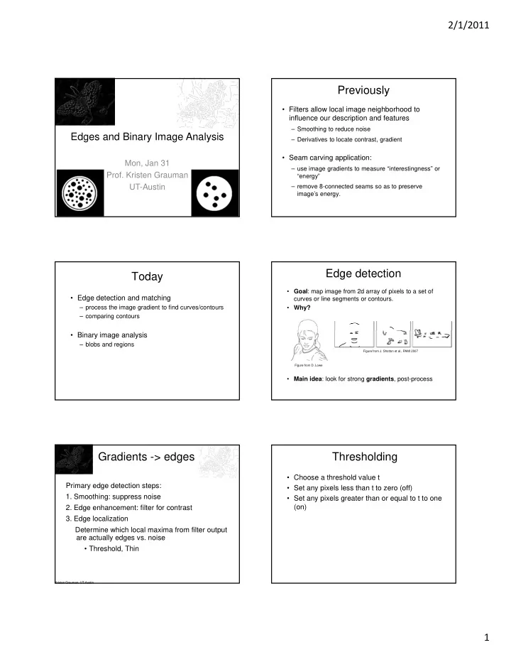
Edge detection

• Goal: map image from 2d array of pixels to a set of

curves or line segments or contours.

• Why?
• Main idea: look for strong gradients, post-process

Figure from J. Shotton et al., PAMI 2007 Figure from D. Lowe

Gradients -> edges

Primary edge detection steps:

• 1. Smoothing: suppress noise
• 2. Edge enhancement: filter for contrast
• 3. Edge localization

Determine which local maxima from filter output are actually edges vs. noise

• Threshold, Thin

Kristen Grauman, UT-Austin

Thresholding

• Choose a threshold value t
• Set any pixels less than t to zero (off)
• Set any pixels greater than or equal to t to one

(on)

2/1/2011 2

Original image Gradient magnitude image Thresholding gradient with a lower threshold Thresholding gradient with a higher threshold

Canny edge detector

• Filter image with derivative of Gaussian
• Find magnitude and orientation of gradient
• Non-maximum suppression:

– Thin wide “ridges” down to single pixel width Linking and thresholding (hysteresis):

• Linking and thresholding (hysteresis):

– Define two thresholds: low and high – Use the high threshold to start edge curves and the low threshold to continue them

• MATLAB: edge(image, ‘canny’);
• >>help edge

Source: D. Lowe, L. Fei-Fei

The Canny edge detector

• riginal image (Lena)

Slide credit: Steve Seitz

2/1/2011 3

The Canny edge detector

norm of the gradient

The Canny edge detector

thresholding

The Canny edge detector

How to turn these thick regions of the gradient into curves? thresholding

Non-maximum suppression

Check if pixel is local maximum along gradient direction, select single max across width of the edge

• requires checking interpolated pixels p and r

The Canny edge detector

Problem:

thinning (non-maximum suppression)

Problem: pixels along this edge didn’t survive the thresholding

Hysteresis thresholding

• Use a high threshold to start edge curves,

and a low threshold to continue them.

Source: Steve Seitz

2/1/2011 4

Hysteresis thresholding

• riginal image
• riginal image

high threshold (strong edges) low threshold (weak edges) hysteresis threshold

Source: L. Fei-Fei

Hysteresis thresholding

• riginal image

high threshold (strong edges) low threshold (weak edges) hysteresis threshold

Source: L. Fei-Fei

Recap: Canny edge detector

• Filter image with derivative of Gaussian
• Find magnitude and orientation of gradient
• Non-maximum suppression:

– Thin wide “ridges” down to single pixel width Linking and thresholding (hysteresis):

• Linking and thresholding (hysteresis):

– Define two thresholds: low and high – Use the high threshold to start edge curves and the low threshold to continue them

• MATLAB: edge(image, ‘canny’);
• >>help edge

Source: D. Lowe, L. Fei-Fei

Low-level edges vs. perceived contours

Background Texture Shadows

Kristen Grauman, UT-Austin

Low-level edges vs. perceived contours

image human segmentation gradient magnitude

Berkeley segmentation database:

http://www.eecs.berkeley.edu/Research/Projects/CS/vision/grouping/segbench/

Source: L. Lazebnik

Learn from humans which combination of features is most indicative of a “good” contour? [D. Martin et al. PAMI 2004]

Human-marked segment boundaries

2/1/2011 5

What features are responsible for perceived edges?

Feature profiles (oriented energy, brightness, color, and texture gradients) along the patch’s [D. Martin et al. PAMI 2004] the patch s horizontal diameter

Kristen Grauman, UT-Austin

What features are responsible for perceived edges?

Feature profiles (oriented energy, brightness, color, and texture gradients) along the patch’s [D. Martin et al. PAMI 2004] the patch s horizontal diameter

Kristen Grauman, UT-Austin

[D. Martin et al. PAMI 2004]

Kristen Grauman, UT-Austin

State-of-the-Art in Contour Detection

Prewitt, Sobel, Roberts Canny Canny+opt thresholds Learned with Human agreement

Computer Vision Group UC Berkeley

Source: Jitendra Malik: http://www.cs.berkeley.edu/~malik/malik-talks-ptrs.html

combined features

Today

• Edge detection and matching

– process the image gradient to find curves/contours – comparing contours

• Binary image analysis

– blobs and regions

Figure from Belongie et al.

2/1/2011 6

Chamfer distance

• Average distance to nearest feature

= I = T

Set of points in image Set of points on (shifted) template

= ) (t dI

Minimum distance between point t and some point in I

Kristen Grauman, UT-Austin

Chamfer distance

Kristen Grauman, UT-Austin

Chamfer distance

• Average distance to nearest feature

How is the measure different than just filtering with a mask having the shape points?

Edge image

points? How expensive is a naïve implementation?

Kristen Grauman, UT-Austin

3 2 2 2 1 2 1 1 2 1 1 1 2 1 2 3 2 1 1 1 1 2 3 3 2 1 1 1 1 1 2 3 4 3 2 1 1 2 2 Distance Transform Image features (2D)

Distance transform

Source: Yuri Boykov

3 4 2 3 2 3 5 4 4 2 2 3 1 1 2 1 1 1 1 2 2

Distance Transform is a function that for each image pixel p assigns a non-negative number corresponding to distance from p to the nearest feature in the image I ) (⋅ D ) (p D

Features could be edge points, foreground points,…

Distance transform

d

• riginal

distance transform edges

Value at (x,y) tells how far that position is from the nearest edge point (or other binary mage structure)

>> help bwdist

Kristen Grauman, UT-Austin

Distance transform (1D)

// 0 if j is in P, infinity otherwise

Adapted from D. Huttenlocher

2/1/2011 7

Distance Transform (2D)

Adapted from D. Huttenlocher

Chamfer distance

• Average distance to nearest feature

Edge image Distance transform image

Kristen Grauman, UT-Austin

Chamfer distance

Fig from D. Gavrila, DAGM 1999

Edge image Distance transform image

Kristen Grauman, UT-Austin

Chamfer distance: properties

• Sensitive to scale and rotation
• Tolerant of small shape changes, clutter
• Need large number of template shapes

g p p

• Inexpensive way to match shapes

Today

• Edge detection and matching

– process the image gradient to find curves/contours – comparing contours

• Binary image analysis

– blobs and regions

Binary images

Kristen Grauman, UT-Austin

2/1/2011 8

Binary image analysis: basic steps

• Convert the image into binary form

– Thresholding

• Clean up the thresholded image

M h l i l t – Morphological operators

• Extract separate blobs

– Connected components

• Describe the blobs with region properties

Kristen Grauman, UT-Austin

Binary images

• Two pixel values

– Foreground and background – Mark region(s) of interest

Thresholding

• Grayscale -> binary mask
• Useful if object of interest’s intensity distribution

is distinct from background

• Example

http://homepages.inf.ed.ac.uk/rbf/CVonline/LOCAL_COPIES/FITZGIBBON/ simplebinary.html

Thresholding

• Given a grayscale image or an intermediate matrix

threshold to create a binary output. Example: edge detection

Gradient magnitude

Looking for pixels where gradient is strong.

fg_pix = find(gradient_mag > t);

Kristen Grauman, UT-Austin

Thresholding

• Given a grayscale image or an intermediate matrix

threshold to create a binary output. Example: background subtraction

=

• Looking for pixels that differ significantly

from the “empty” background.

fg_pix = find(diff > t);

Kristen Grauman, UT-Austin

Thresholding

• Given a grayscale image or an intermediate matrix

threshold to create a binary output. Example: intensity-based detection

Looking for dark pixels

fg_pix = find(im < 65);

Kristen Grauman, UT-Austin

2/1/2011 9

Thresholding

• Given a grayscale image or an intermediate matrix

threshold to create a binary output. Example: color-based detection

Looking for pixels within a certain hue range.

fg_pix = find(hue > t1 & hue < t2);

Kristen Grauman, UT-Austin

A nice case: bimodal intensity histograms

Ideal histogram, light object on dark background Actual observed histogram with noise

Images: http://homepages.inf.ed.ac.uk/rbf/CVonline/LOCAL_COPIES/OWENS/LECT2/node3.html

Not so nice cases

Shapiro and Stockman

Issues

• What to do with “noisy” binary
• utputs?

– Holes – Extra small fragments

• How to demarcate multiple

regions of interest?

– Count objects – Compute further features per

• bject

Kristen Grauman, UT-Austin

Morphological operators

• Change the shape of the foreground regions via

intersection/union operations between a scanning structuring element and binary image.

• Useful to clean up result from thresholding
• Useful to clean up result from thresholding
• Basic operators are:

– Dilation – Erosion

Dilation

• Expands connected components
• Grow features
• Fill holes

Before dilation After dilation

Kristen Grauman, UT-Austin

2/1/2011 10

Erosion

• Erode connected components
• Shrink features
• Remove bridges, branches, noise

Before erosion After erosion

Kristen Grauman, UT-Austin

Structuring elements

• Masks of varying shapes and sizes used to

perform morphology, for example:

• Scan mask across foreground pixels to

transform the binary image

>> help strel

Kristen Grauman, UT-Austin

Dilation vs. Erosion

At each position:

• Dilation: if current pixel is foreground, OR the

structuring element with the input image.

Example for Dilation (1D)

SE x f x g ⊕ ) ( ) (

1 1 1 1 1 1

Input image Structuring Element

1 1 1

SE x f x g ⊕ = ) ( ) (

1 1

Output Image

Adapted from T. Moeslund

Example for Dilation

1 1 1 1 1 1

Input image St t i El t

1 1 1

Structuring Element

1 1

Output Image

1 1 1

Example for Dilation

1 1 1 1 1 1

Input image St t i El t

1 1 1

Structuring Element

1 1

Output Image

1 1 1

2/1/2011 11

Example for Dilation

1 1 1 1 1 1

Input image St t i El t

1 1 1

Structuring Element

1 1

Output Image

1 1 1

Example for Dilation

1 1 1 1 1 1

Input image St t i El t

1 1 1

Structuring Element

1 1 1 1 1

Output Image

1 1 1

Example for Dilation

1 1 1 1 1 1

Input image St t i El t

1 1 1

Structuring Element

1 1 1 1 1 1

Output Image

1 1 1

Example for Dilation

1 1 1 1 1 1

Input image St t i El t

1 1 1

Structuring Element

1 1 1 1 1 1 1

Output Image

1 1 1

Example for Dilation

1 1 1 1 1 1

Input image St t i El t

1 1 1

Structuring Element

1 1 1 1 1 1 1

Output Image

1 1 1

Example for Dilation

1 1 1 1 1 1

Input image St t i El t

1 1 1

Structuring Element

1 1 1 1 1 1 1 1 1

Output Image

1 1 1

Note that the object gets bigger and holes are filled.

>> help imdilate

2/1/2011 12

2D example for dilation

Shapiro & Stockman

Dilation vs. Erosion

At each position:

• Dilation: if current pixel is foreground, OR

the structuring element with the input image.

• Erosion: if every pixel under the structuring

element’s nonzero entries is foreground, OR g , the current pixel with S.

Example for Erosion (1D)

1 1 1 1 1 1

Input image St t i El t

1 1 1

Structuring Element Output Image

SE x f x g O ) ( ) ( =

_

Example for Erosion (1D)

1 1 1 1 1 1

Input image St t i El t

1 1 1

Structuring Element Output Image

SE x f x g O ) ( ) ( =

_

Example for Erosion

1 1 1 1 1 1

Input image St t i El t

1 1 1

Structuring Element Output Image

1 1 1

Example for Erosion

1 1 1 1 1 1

Input image St t i El t

1 1 1

Structuring Element Output Image

1 1 1

2/1/2011 13

Example for Erosion

1 1 1 1 1 1

Input image St t i El t

1 1 1

Structuring Element Output Image

1 1 1

Example for Erosion

1 1 1 1 1 1

Input image St t i El t

1 1 1

Structuring Element

1

Output Image

1 1 1

Example for Erosion

1 1 1 1 1 1

Input image St t i El t

1 1 1

Structuring Element

1

Output Image

1 1 1

Example for Erosion

1 1 1 1 1 1

Input image St t i El t

1 1 1

Structuring Element

1

Output Image

1 1 1

Example for Erosion

1 1 1 1 1 1

Input image St t i El t

1 1 1

Structuring Element

1

Output Image

1 1 1

Example for Erosion

1 1 1 1 1 1

Input image St t i El t

1 1 1

Structuring Element

1 1

Output Image

1 1 1

Note that the object gets smaller

>> help imerode

2/1/2011 14

2D example for erosion

Shapiro & Stockman

Opening

• Erode, then dilate
• Remove small objects, keep original shape

Before opening After opening

Closing

• Dilate, then erode
• Fill holes, but keep original shape

Before closing After closing Applet: http://bigwww.epfl.ch/demo/jmorpho/start.php

Morphology operators on grayscale images

• Dilation and erosion typically performed on binary

images.

• If image is grayscale: for dilation take the

neighborhood max, for erosion take the min. g

• riginal

dilated eroded

Kristen Grauman, UT-Austin

Issues

• What to do with “noisy” binary
• utputs?

– Holes – Extra small fragments

• How to demarcate multiple

regions of interest?

– Count objects – Compute further features per

• bject

Kristen Grauman, UT-Austin

Connected components

• Various algorithms to compute

– Recursive (in memory) – Two rows at a time (image not necessarily in memory) memory) – Parallel propagation strategy

2/1/2011 15

Recursive connected components

• Find an unlabeled pixel, assign it a new

label

• Search to find its neighbors, and

recursively repeat to find their neighbors til

• Demo http://www.cosc.canterbury.ac.nz/mukundan/covn/Label.html

recursively repeat to find their neighbors til there are no more

• Repeat

Connected components

• Identify distinct regions of “connected pixels”

Shapiro and Stockman

Connectedness

• Defining which pixels are considered neighbors

4-connected 8-connected

Source: Chaitanya Chandra

Connected components

• We’ll consider a sequential

algorithm that requires only 2 passes over the image.

• Input: binary image
• Input: binary image
• Output: “label” image,

where pixels are numbered per their component

• Note: foreground here is

denoted with black pixels.

Sequential connected components

Adapted from J. Neira

Sequential connected components

2/1/2011 16

Sequential connected components Sequential connected components Connected components

Slide credit: Pinar Duygulu

Region properties

• Given connected components, can compute

simple features per blob, such as:

– Area (num pixels in the region) – Centroid (average x and y position of pixels in the region) – Bounding box (min and max coordinates) Circularity (ratio of mean dist to centroid over std) – Circularity (ratio of mean dist. to centroid over std)

A1=200 A2=170

Kristen Grauman, UT-Austin

Circularity

Shapiro & Stockman [Haralick]

Binary image analysis: basic steps (recap)

• Convert the image into binary form

– Thresholding

• Clean up the thresholded image

M h l i l t – Morphological operators

• Extract separate blobs

– Connected components

• Describe the blobs with region properties

2/1/2011 17

Matlab

• N = hist(Y,M)
• L = bwlabel (BW,N);
• STATS = regionprops(L,PROPERTIES) ;

– 'Area' – 'Centroid' 'BoundingBox' – 'BoundingBox' – 'Orientation‘, …

• IM2 = imerode(IM,SE);
• IM2 = imdilate(IM,SE);
• IM2 = imclose(IM, SE);
• IM2 = imopen(IM, SE);

Example using binary image analysis: OCR

[Luis von Ahn et al. http://recaptcha.net/learnmore.html]

Example using binary image analysis: segmentation of a liver

Slide credit: Li Shen

Example using binary image analysis: Bg subtraction + blob detection

…

Example using binary image analysis: Bg subtraction + blob detection

University of Southern California http://iris.usc.edu/~icohen/projects/vace/detection.htm

Binary images

• Pros

– Can be fast to compute, easy to store – Simple processing techniques available – Lead to some useful compact shape descriptors

• Cons

– Hard to get “clean” silhouettes – Noise common in realistic scenarios – Can be too coarse of a representation – Not 3d

Kristen Grauman, UT-Austin

2/1/2011 18

Summary

• Operations, tools

Derivative filters Smoothing, morphology Thresholding Connected components Matched filters Histograms

• Features,

representations

Edges, gradients Blobs/regions Local patterns Textures (next) Color distributions Histograms

Next

• Texture: read 10.5
• Pset 1 out tonight, due in 2 weeks