Preserving Confidentiality Overview AND Providing Adequate Data - - PowerPoint PPT Presentation

Page 1

1

Preserving Confidentiality AND Providing Adequate Data for Statistical Modeling

Stephen E. Fienberg

Department of Statistics Center for Automated Learning and Discovery Center for Computer and Communications Security Carnegie Mellon University Pittsburgh, PA, U.S.A.

2

Overview

• Background and some fundamental

abstractions for disclosure limitation.

– Statistical users want more than to retrieve a few numbers.

• Results on bounds for table entries.
• Uses of Markov bases for exact

distributions and perturbation of tables.

• Links to log-linear models, and related

statistical theory and methods.

3

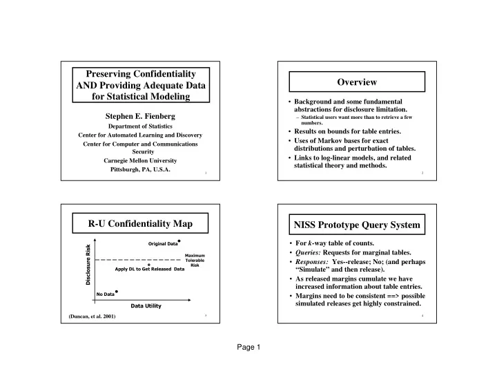
R-U Confidentiality Map

• (Duncan, et al. 2001)

4

• For k-way table of counts.
• Queries: Requests for marginal tables.
• Responses: Yes--release; No; (and perhaps

“Simulate” and then release).

• As released margins cumulate we have

increased information about table entries.

• Margins need to be consistent ==> possible

simulated releases get highly constrained.

NISS Prototype Query System

Page 2

5

Confidentiality Concern

• Uniqueness in population table ⇔

⇔ ⇔ ⇔ cell count of “1”.

• Uniqueness allows intruder to match

characteristics in table with other data bases that include the same variables plus

• thers to learn confidential information.

– Assuming data are reported without error!

• Identity versus attribute disclosure.

6

• Query space, Q, with partial ordering:

– Elements can be marginal tables, conditionals, k- groupings, regressions, or other data summaries. – Released set: R(t), and implied Unreleasable set: U(t). – Releasable frontier: maximal elements of R(t). – Unreleasable frontier: minimal elements of U(t).

• Risk and Utility defined on subsets of Q.

– Risk Measure: identifiability of small cell counts. – Utility: reconstructing table using log-linear models. – Release rules must balance risk and utility:

• R-U Confidentiality map.
• General Bayesian decision-theoretic approach.

Fundamental Abstractions

7

Why Marginals?

• Simple summaries corresponding to

subsets of variables.

• Traditional mode of reporting for

statistical agencies and others.

• Useful in statistical modeling: Role of

log-linear models.

• Collapsing categories of categorical

variables uses similar DL methods and statistical theory.

8

Example 1: 2000 Census

• U.S. decennial census “long form”

– 1 in 6 sample of households nationwide. – 53 questions, many with multiple categories. – Data measured with substantial error! – Data reported after application of data swapping!

• Geography

– 50 states; 3,000 counties; 4 million “blocks”. – Release of detailed geography yields uniqueness in sample and at some level in population.

• American Factfinder releases various 3-way

tables at different levels of geography.

Page 3

9 10

Example 2: Risk Factors for Coronary Heart Disease

• 1841 Czech auto workers

Edwards and Havanek (1985)

• 26 table
• population data

– “0” cell

– population unique, “1” – 2 cells with “2”

Smoke (Y/ N) Me nta l work P hys. work

• Syst. BP

Lipo ra tio Ana mne sis a b c d e f 11

Example 2: The Data

B no yes F E D C A no yes no yes ne g < 3 < 140 no 44 40 112 67 yes 129 145 12 23 ≥ ≥ ≥ ≥ 140 no 35 12 80 33 yes 109 67 7 9 ≥ ≥ ≥ ≥ 3 < 140 no 23 32 70 66 yes 50 80 7 13 ≥ ≥ ≥ ≥ 140 no 24 25 73 57 yes 51 63 7 16 pos < 3 < 140 no 5 7 21 9 yes 9 17 1 4 ≥ ≥ ≥ ≥ 140 no 4 3 11 8 yes 14 17 5 2 ≥ ≥ ≥ ≥ 3 < 140 no 7 3 14 14 yes 9 16 2 3 ≥ ≥ ≥ ≥ 140 no 4 13 11 yes 5 14 4 4

12

Example 3: NLTCS

• National Long Term Care Survey

– 20-40 demographic/background items. – 30-50 items on disability status, ADLs and IADLs, most binary but some polytomous. – Linked Medicare files. – 5 waves: 1982, 1984, 1989, 1994, 1999.

• We’ve been working with 216 table,

collapsed across several waves of survey, with n=21,574.

Erosheva (2002) Dobra, Erosheva, & Fienberg(2003)

Page 4

13

• For 2×

× × ×2 tables of counts{nij} given the marginal totals {n1+,n2+} and {n+1,n+2}:

• Interested in multi-way generalizations

involving higher-order, overlapping margins.

Two-Way Fréchet Bounds

) , max( ) , min(

2 1 2 22 21 1 12 11

n n n n n n n n n n n n n n n

j i ij j i

− − − − + + + + ≥ ≥ ≥ ≥ ≥ ≥ ≥ ≥

+ + + + + + + + + + + + + + + + + + + + + + + + + + + + + + + +

14

• k-way table of non-negative counts, k ≥

≥ ≥ ≥ 3.

– Release set of marginal totals, possibly overlapping. – Goal: Compute bounds for cell entries. – LP and IP approaches are NP-hard.

• Our strategy has been to:

– Develop efficient methods for several special cases. – Exploit linkage to statistical theory where possible. – Use general, less efficient methods for residual cases.

• Direct generalizations to tables with non-

integer, non-negative entries.

Bounds for Multi-Way Tables

15

• For 2×

× × ×2 case, lower bound is evocative of MLE for estimated expected value under independence:

– Bounds correspond to log-linearized version. – Margins are minimal sufficient statistics (MSS).

. / ˆ n n n m

j i ij + + + + + + + +

= = = =

) ( 23 ) ( 13 ) ( 12 ) ( 3 ) ( 2 ) ( 1

) log(

jk ik ij k j i ijk

u u u u u u u m + + + + + + + + + + + + + + + + + + + + + + + + = = = =

Role of Log-linear Models?

• In 3-way table of counts, {nijk}, we model logs
• f expectations {E(nijk)=mijk}:
• MSS are margins corresponding to highest order

terms: {nij+}, {ni+k}, {n+jk}.

16

Graphical & Decomposable Log-linear Models

• Graphical models: defined by simultaneous

conditional independence relationships

– Absence of edges in graph.

Example 2: Czech autoworkers Graph has 3 cliques: [ADE][ABCE][BF]

• Decomposable models correspond to

triangulated graphs.

Smoke (Y/ N) Mental work P hys. work S yst. BP Lipo ratio Ana a b c d e f

Page 5

17

MLEs for Decomposable Log-linear Models

• For decomposable models, expected cell

values are explicit function of margins, corresponding to MSSs (cliques in graph):

– For conditional independence in 3-way table:

• Substitute observed margins for expected

in explicit formula to get MLEs.

logmijk = = = = u + + + + u1(i) + + + + u2( j) + + + + u3(k) + + + + u12(ij) + + + + u13(ik)

mijk = = = =

mij+ + + +mi+ + + +k mi+ + + ++ + + +

18

Multi-way Bounds

• For decomposable log-linear models:
• Theorem: When released margins

correspond to those of a decomposable model:

– Upper bound: minimum of relevant margins. – Lower bound: maximum of zero, or sum of relevant margins minus separators. – Bounds are sharp.

Fienberg and Dobra (2000)

∏ ∏ ∏ ∏ ∏ ∏ ∏ ∏

= = = = Separators MSSs Value Expected

19

• Example: Given margins in k-way table

that correspond to (k-1)-fold conditional independence given variable 1:

• Then bounds are

} ), 2 ( ... max{ } ,..., , min{

... ... ... ... ... ... ...

3 ... 1 3 1 2 1 3 2 1 1 3 1 2 1

− − − − − − − − + + + + + + + + + + + + ≥ ≥ ≥ ≥ ≥ ≥ ≥ ≥

+ + + + + + + + + + + + + + + + + + + + + + + + + + + + + + + + + + + + + + + + + + + + + + + + + + + + + + + + + + + + + + + + + + + + + + + +

+ + + + + + + +

k n n n n n n n n

i i i i i i i i i i i i i i i

k i i k k

} { .... } { } {

... ... ...

1 3 1 2 1 k

i i i i i i

n n n

+ + + + + + + + + + + + + + + + + + + + + + + +

Multi-Way Bounds (cont.)

20

• Ex. 2: Czech Autoworkers
• Suppose released margins are

[ADE][ABCE][BF] :

– Correspond to decomposable graph. – Cell containing population unique has bounds [0, 25]. – Cells with entry of “2” have bounds: [0,20] and [0,38]. – Lower bounds are all “0”.

• “Safe” to release these margins; low risk
• f disclosure.

S moke (Y/ N) Menta l work P hys. work

• Syst. BP

Lipo ra tio Anamne sis a b c d e f

Page 6

21

Bounds for [BF][ABCE][ADE]

B no yes F E D C A no yes no yes neg < 3 < 140 no [0,88] [0,62] [0,224] [0,117] yes [0,261] [0,246] [0,25] [0,38] ≥ ≥ ≥ ≥ 140 no [0,88] [0,62] [0,224] [0,117] yes [0,261] [0,151] [0,25] [0,38] ≥ ≥ ≥ ≥ 3 < 140 no [0,58] [0,60] [0,170] [0,148] yes [0,115] [0,173] [0,20] [0,36] ≥ ≥ ≥ ≥ 140 no [0,58] [0,60] [0,170] [0,148] yes [0,115] [0,173] [0,20] [0,36] pos < 3 < 140 no [0,88] [0,62] [0,126] [0,117] yes [0,134] [0,134] [0,25] [0,38] ≥ ≥ ≥ ≥ 140 no [0,88] [0,62] [0,126] [0,117] yes [0,134] [0,134] [0,25] [0,38] ≥ ≥ ≥ ≥ 3 < 140 no [0,58] [0,60] [0,126] [0,126] yes [0,115] [0,134] [0,20] [0,36] ≥ ≥ ≥ ≥ 140 no [0,58] [0,60] [0,126] [0,126] yes [0,115] [0,134] [0,20] [0,36]

Table 1 - Bounds for Autoworkers data given the marginals [BF], [ABCE], [ADE]. 22

Example 2 (cont.)

• Among all 32,000+ decomposable models,

the tightest possible bounds for three target cells are: (0,3), (0,6), (0,3).

– 31 models with these bounds! All involve [ACDEF]. – Another 30 models have bounds that differ by 5 or less (critical width) and these involve [ABCDE]. – Method used to search for “optimal” decomposable release also identifies [ABDEF] as potentially problematic.

• Allows proper statistical test of fit for most

interesting models.

23

• Extension for log-linear models and margins

corresponding to reducible graphs.

• For 2k tables with (k-1) dimensional margins fixed

(need one extra bound here and it comes from log-linear model theory: existence of MLEs).

– Extend to general k-way case by looking at all possible collapsed 2k tables.

• General “shuttle” algorithm in Dobra (2002)

works for all cases.

– Also generates most special cases with limited extra computation.

More on Bounds

24

Example 2: Release of All 5-way Margins

• Approach for 2×

× × ×2× × × ×2 generalizes to 2k table given (k-1)-way margins.

• In 26 table, if we release all 5-way

margins:

– Almost identical upper and lower values; they all differ by 1. – Only 2 feasible tables with these margins!

• UNSAFE!

Page 7

25

Example 3: NLTCS

• 216 table of ADL/IADLs with 65,536 cells:

– 62,384 zero entries; 1,729 cells with count of “1” and 499 cells with count of “2”. – n=21,574. – Largest cell count: 3,853---no disabilities.

• Used simulated annealing algorithm to

search all decomposable models for “decomposable” model on frontier with max[upper bound – lower bound] >3.

• Acting as if these were population data.

26

• Decomposable frontier model:

{[1,2,3,4,5,7,12], [1,2,3,6,7,12], [2,3,4,5,7,8], [1,2,4,5,7,11], [2,3,4,5,7,13], [3,4,5,7,9,13], [2,3,4,5,13,14], [2,4,5,10,13,14], [1,2,3,4,5,15], [2,3,4,5,8,16]}.

• Has one 7-way and eight 6-way marginals.

NLTCS Search Results Perturbation Maintaining Marginal Totals

v1 v2 v3 v4 w1 w2 w3 w4

+1 –1 +1 –1

• Perturbation distributions given marginals require

Markov basis for perturbation moves.

28

• Perturbation preserving marginals

involves a parallel set of results to those for bounds:

– Markov basis elements for decomposable case requires only “simple” moves. (Dobra, 2002) – Efficient generation of Markov basis for reducible

• case. (Dobra and Sullivent, 2002)

– Simplifications for 2k tables (“binomials”). – Rooted in ideas from likelihood theory for log-linear models and computational algebra of toric ideals.

Perturbation for Protection

Page 8

29

Some Ongoing Research

• Queries in form of combinations of

marginals and conditionals.

• Inferences from marginal releases.
• What information does the intruder

really have?

• Record linkage and matching.
• Simplified cyclic perturbation

distributions.

• Computational algebraic statistics.

30

Summary

• Some fundamental abstractions for

disclosure limitation.

• Results on bounds for table entries.
• Parallels for Markov bases for exact

distributions and perturbation of tables.

• New theoretical links among disclosure

limitation, statistical theory, and computational algebraic geometry.

31

The End

• Most papers available for downloading at

http://www.niss.org http://www.stat.cmu.edu/~fienberg/disclosure.html

• Workshop on Computational Algebraic Statistics

December 14 to 18, 2003, American Institute of Mathematics, Palo Alto, California http://aimath.org/ARCC/workshops/compalgstat.html

32

Stochastic Perturbation Methods

• Some methods well-developed in

statistical literature:

– Matrix masking, including adding noise – Post-randomization

• Randomized response after data are collected

– Multiple Imputation

• Sampling from full posterior distribution

– Data swapping and constrained cyclic perturbation

• Key is full information on stochastic

transformation for proper statistical inferences.

Page 9

33

Exact Distribution of Table Given Marginals

• Exact probability distribution for log-

linear model given its MSS marginals:

– Can generate distribution using Diaconis-Sturmfels (1998) MCMC approach using Markov basis. Fienberg, Makov, Meyer, Steele (2002)

• ∏

∏ ∏ ∏ ∏ ∏ ∏ ∏

∈ ∈ ∈ ∈ ∈ ∈ ∈ ∈ ∈ ∈ ∈ ∈

• =

= = =

) (

)! ( 1 )! ( 1 ) n (

c S m I i I i

i m i n σ σ σ σ

34

Markov Basis “Moves”

• Simple moves:

– Based on standard linear contrasts involving 1’s, 0’s, and -1’s for embedded 2l subtables. – For example, in 2×2×2 table, there is 1 move of form:

• “Non-simple” moves:

– Require combination of simple moves to reach extremal tables in convex polytope.

1 -1

• 1

1

• 1

1 1

• 1

35

Challenge: Scaling up approach for large k.

Three-way Illustration (k=3)

36

NISS Table Server: 6-Way Table