Preface Face Recognition Haibin Ling Many slides revised from K. - - PDF document

1

CIS 5543 – Computer Vision

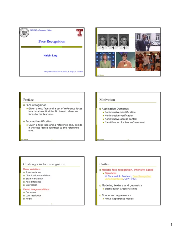
Face Recognition

Haibin Ling

Many slides revised from K. Grosse, R. Fergus, S. Lazebnik

Karl Grosse

Preface

Karl Grosse 3

Preface

 Face recognition  Given a test face and a set of reference faces

in a database find the N closest reference faces to the test one.

 Face authentification  Given a test face and a reference one, decide

if the test face is identical to the reference

• ne.

Karl Grosse 4

Motivation

 Application Demands  Nonintrusive identification  Nonintrusive verification  Nonintrusive access control  Identification for law enforcement

5

Challenges in face recognition

Many variations

 Pose variation  Illumination conditions  Scale variability  Age difference  Expression

Varied image conditions

 Occlusion  Low resolution  Noise

Outline

 Holistic face recognition, intensity based

 Eigenfaces

• M. Turk and A. Pentland, Face Recognition

using Eigenfaces, CVPR 1991

 Modeling texture and geometry

 Elastic Bunch Graph Matching

 Shape and appearance

 Active Appearance models

2 Principal Component Analysis

• Given: N data points x1, … ,xN in Rd
• We want to find a new set of features that

are linear combinations of original ones: u(xi) = uT(xi – µ) (µ: mean of data points)

• What unit vector u in Rd captures the

most variance of the data?

Projection of data point Covariance matrix of data

N N

Principal Component Analysis

• Direction that maximizes the variance of the

projected data:

The direction that maximizes the variance is the eigenvector associated with the largest eigenvalue of Σ

Eigenfaces: Key idea

• Assume that most face images lie on a low-

dimensional subspace determined by the first k (k<d) directions of maximum variance

• Use PCA to determine the vectors u1,…uk that

span that subspace: x ≈ μ + w1u1 + w2u2 + … + wkuk

• Represent each face using its “face space”

coordinates (w1,…wk)

• Perform nearest-neighbor recognition in “face

space”

• M. Turk and A. Pentland, Face Recognition using Eigenfaces, CVPR 1991

Eigenface examples

 Training

images

 x1,…,xN

Eigenface example

Top eigenvectors: u1,…uk Mean: μ

Eigenfaces example

• Face x in “face space” coordinates:

=

3 Eigenfaces example

• Face x in “face space” coordinates:

Reconstruction:

=

= + µ + w1u1+w2u2+w3u3+w4u4+ … ^ x =

Summary: Recognition with eigenfaces

 Process labeled training images:

• Find mean µ and covariance matrix Σ
• Find k principal components (eigenvectors of Σ) u1,…uk
• Project each training image xi onto subspace spanned by

principal components: (wi1,…,wik) = (u1

T(xi – µ), … , uk T(xi – µ))

 Given novel image x:

• Project onto subspace:

(w1,…,wk) = (u1

T(x – µ), … , uk T(x – µ))

• Optional: check reconstruction error x – x to determine

whether image is really a face

• Classify as closest training face in k-dimensional subspace

^

Limitations

• Global appearance method: not robust to

misalignment, background variation

Limitations

• PCA assumes that the data has a Gaussian

distribution (mean µ, covariance matrix Σ)

The shape of this dataset is not well described by its principal components

Other Component Analysis

• Is principle component the right one?
• Direction of maximum variance good for classification?
• More subspace methods:
• Fisherfaces (LDA, Belhumeur et al. 1997)
• Independent Component Analysis (ICA, Bartlett et al. 2002)
• Nonlinear embedding
• Laplacian face (LPP, He et al. 2005)

Outline

 Holistic face recognition, intensity based

 Eigenfaces

 Shape and appearance

 Active Appearance models

Cootes, Edwards, and Taylor, “Active Appearance Models”, ECCV 1998  Modeling texture and geometry

 Elastic Bunch Graph Matching

4

Essence of the Idea: Recognition by Synthesis

 Explain a new example in terms of the model parameters Slide: Dhruv Batra

So what’s a model

Model “Shape” “texture” Slide: Dhruv Batra

Active Shape Models

training set Slide: Dhruv Batra

Shape Vector

= 43 Provides alignment!

Slide: Dhruv Batra

Texture Models

warp to mean shape

Slide: Dhruv Batra

The Morphable Face Model

Shape S Appearance T

Cootes, Edwards, and Taylor, “Active Appearance Models”, ECCV 1998

The structure of a face

 Shape vector

S = (x1, y1, x2, … , yn) T, containing the (x,y) coordinates of vertices of a face,

 Appearance vector T = (R1, G1, B1, R2, …

, Gn, Bn) T, containing the color values of the mean-warped face image.

5

The Morphable face model



Again, assuming that we have m such vector pairs in full correspondence, we can form new shapes Smodel and new appearances Tmodel as:



If number of basis faces m is large enough to span the face subspace then:



Any new face can be represented as a pair of vectors (1, 2m) T and (1, 2m) T !







m i i i model

a

1

S S







m i i i model

b

1

T T

Active Appearance Model Search (Results)

Slide: Dhruv Batra

Playing with the Parameters

First two modes of shape variation First two modes of gray-level variation First four modes of appearance variation

Slide: Dhruv Batra

Overview

 Holistic face recognition, intensity based

 Eigenfaces

 Shape and appearance

 Active Appearance models

 Modeling texture and geometry

 Elastic Bunch Graph Matching

• L. Wiskott, J.M. Fellouse, N. Krüger, C.v.d.Malsburg Face

Recognition by Elastic Bunch Graph Matching, PAMI 1997

Karl Grosse

EBGM Overview

 Human faces share a similar topological structure  Labeled graph as basic object representation

 Nodes positioned at fiducial points (eyes, nose…)  Jets at each node  Edges labeled with distance information

 Stored model graph matched to new images

Image graph (can become model graph)

 Model graphs easily translated, scaled, orientated

Karl Grosse

Gabor wavelets

 Shape of plane waves

restricted by a Gaussian envelope function

 Hence good results in practice  Biologically motivated

Pro: Invariant to changes in brightness Robust against translation or distortion Con: Dependent on the background of the image

6

Karl Grosse

Gabor wavelets

Family of Gabor kernels In the shape of plane waves with wave vector restricted by a Gaussian envelope function. 5 different frequencies 8 orientations Width of Gaussian controlled by Family of kernels is self-similar and generated from one mother wavelet by dilation and rotation!

Karl Grosse

Jets

 Wavelets for different frequencies and orientation  Jet describes a small patch of grey values  Defined as the set of complex coefficients

J={Ji} for a given pixel

Karl Grosse

Image graph

 Image Graph G: N nodes, E edges  Labeling of nodes:

Jets Jn at positions xn, n = 1,…, N

 Labeling of edges:

Distances between nodes n and n´

 Graph is not complete

Karl Grosse

Bunch graph

Constructing a Bunch graph B from M Image graphs GBM:

 Summarize the jets from a node

Set of jets “Bunch”

 Label nodes with Bunches  Label edges with average distance

Karl Grosse

Matching



Goal: Calculate an Image graph for an image

• Four stages:

1.

Find approximate position

2.

Refine position and size

3.

Refine size and find aspect ratio

4.

Local distortion



Initial Graph: Structure of Bunch Graph

Karl Grosse

Matching

Image graphs found by probing with the Bunch graph

7

Karl Grosse

Matching

Top row: Image graphs manually marked Bottom row: Image graphs found by the system

Karl Grosse

Comparison of results

 Results of face recognition using the FERET db:

 Different poses: frontal, halfprofile, profile

Conclusion

 Holistic face recognition  Assuming faces are aligned  Subspace approach  Active shape/appearance model  Separate shape and appearance  Landmark based face warping  Elastic Bunch Graph Matching  Modeling topological with a graph  Modeling local appearance with Gabor  Open problems  Alignment  Occlusion and cluttering  Expression, aging, glasses, facial hair