Face detection and recognition Many slides adapted from K. Grauman - - PowerPoint PPT Presentation

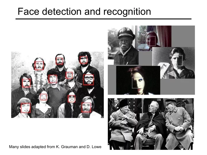
Face detection and recognition

Many slides adapted from K. Grauman and D. Lowe

Face detection and recognition

Detection Recognition

“Sally”

Consumer application: iPhoto 2009

http://www.apple.com/ilife/iphoto/

Consumer application: iPhoto 2009

Can be trained to recognize pets!

http://www.maclife.com/article/news/iphotos_faces_recognizes_cats

Consumer application: iPhoto 2009

Things iPhoto thinks are faces

Outline

• Face recognition
• Eigenfaces
• Face detection
• The Viola & Jones system

The space of all face images

• When viewed as vectors of pixel values, face

images are extremely high-dimensional

• 100x100 image = 10,000 dimensions
• However, relatively few 10,000-dimensional

vectors correspond to valid face images

• We want to effectively model the subspace of

face images

The space of all face images

• We want to construct a low-dimensional linear

subspace that best explains the variation in the set of face images

Principal Component Analysis

• Given: N data points x1, … ,xN in Rd
• We want to find a new set of features that are

linear combinations of original ones: u(xi) = uT(xi – µ) (µ: mean of data points)

• What unit vector u in Rd captures the most

variance of the data?

Forsyth & Ponce, Sec. 22.3.1, 22.3.2

Principal Component Analysis

• Direction that maximizes the variance of the projected data:

Projection of data point Covariance matrix of data

The direction that maximizes the variance is the eigenvector associated with the largest eigenvalue of Σ N N

Principal component analysis

• The direction that captures the maximum

covariance of the data is the eigenvector corresponding to the largest eigenvalue of the data covariance matrix

• Furthermore, the top k orthogonal directions

that capture the most variance of the data are the k eigenvectors corresponding to the k largest eigenvalues

Eigenfaces: Key idea

• Assume that most face images lie on

a low-dimensional subspace determined by the first k (k<d) directions of maximum variance

• Use PCA to determine the vectors or

“eigenfaces” u1,…uk that span that subspace

• Represent all face images in the dataset as

linear combinations of eigenfaces

• M. Turk and A. Pentland, Face Recognition using Eigenfaces, CVPR 1991

Eigenfaces example

Training images x1,…,xN

Eigenfaces example

Top eigenvectors: u1,…uk Mean: μ

Eigenfaces example

Principal component (eigenvector) uk μ + 3σkuk μ – 3σkuk

Eigenfaces example

• Face x in “face space” coordinates:

=

Eigenfaces example

• Face x in “face space” coordinates:
• Reconstruction:

= + µ + w1u1+w2u2+w3u3+w4u4+ …

=

^ x =

Reconstruction demo

Recognition with eigenfaces

Process labeled training images:

• Find mean µ and covariance matrix Σ
• Find k principal components (eigenvectors of Σ) u1,…uk
• Project each training image xi onto subspace spanned by

principal components: (wi1,…,wik) = (u1

T(xi – µ), … , uk T(xi – µ))

Given novel image x:

• Project onto subspace:

(w1,…,wk) = (u1

T(x – µ), … , uk T(x – µ))

• Optional: check reconstruction error x – x to determine

whether image is really a face

• Classify as closest training face in k-dimensional

subspace ^

• M. Turk and A. Pentland, Face Recognition using Eigenfaces, CVPR 1991

Recognition demo

Limitations

• Global appearance method: not robust to

misalignment, background variation

Limitations

• PCA assumes that the data has a Gaussian

distribution (mean µ, covariance matrix Σ)

The shape of this dataset is not well described by its principal components

Limitations

• The direction of maximum variance is not

always good for classification