Predictor-Corrector and Morphing Ensemble Filters for the Assimilation of Sparse Data into High-Dimensional Nonlinear Systems Jan Mandel and Jonathan D. Beezley University of Colorado and National Center for Atmospheric Research American Meteorological Society Annual Meeting San Antonio, TX, January 16, 2007 Supported by National Science Foundation Grant CNS-0325314 and NCAR faculty fellowship.
Data Assimilation for Highly Nonlinear Problems • Coherent features: fireline in wildfire, hurricane vortex • Error in position of feature typically have close to Gaussian distribution • Error in physical fields at a fixed point typically do not - multimodal – wildfire: concentrated about burning/not burning – hurricane: which side of the vortex are we on? • The closer to Gaussian the better ⇒ transformation of variables to get closer to Gaussian: Morphing Filters • EnKF based on the Gaussian assumption ⇒ combine with particle filters: Predictor-Corrector Filters
1. Morphing Ensemble Filters
Data Assimilation and Additive vs Positional Correction • alternative error models including the position of features (Hoffman et al., 1995) • additive correction to spatial transformation instead of original variables – global low order polynomial mapping for alignment (Alexander et al., 1998) – alignment as preprocessing to an additive correction (Lawson and Hansen, 2005; Ravela et al., 2006) • New Morphing Filter: a one-step method – additive correction to spatial transformation and variable values – by automatic image registration, borrowed from image processing
Intermediate States by Morphing Registration Given two functions u 0 and u 1 , find transformation U such that � u 1 − u 0 ◦ ( I + T ) � + C 1 � T � + C 2 � ▽ T � → min . for suitable norms and constants (Gao, 1998), with modifications to speed up and decrease the chances of getting stuck in a local minimum. Create intermediate functions u λ between u 0 and u 1 , by r = u 1 ◦ ( I + T ) − 1 − u 0 u λ = ( u 0 + λr ) ◦ ( I + λT ) , 0 ≤ λ ≤ 1 , Morphing Ensemble Kalman Filter The EnKF is least squares on linear combinations of ensemble members. Fix u 0 and replace linear combinations by morphing: apply EnKF to the morphing representation [ r, T ]
Intermediate States by Morphing λ = 0 λ = 0 . 25 λ = 0 . 5 λ = 0 . 75 λ = 1 Morphing of two solutions of a reaction-diffusion equation system used in a wildfire simulation. The states with λ = 0 and λ = 1 are given. The intermediate states are created automatically. The horizontal plane is the earth surface. The vertical axis and the color map are the temperature. The morphing algorithm combines the values as well as the positions.
Data assimilation by the Morphing Ensemble Kalman Filter (a) (b) (c) (d) The forecast ensemble (b) was created by smooth random morphing of the initial temperature profile (a). The analysis ensemble (d) was obtained by the EnKF applied to the transformed state. The data for the EnKF was the morphing transformation of the simulated data (c), and the observation function was the identity mapping. Contours are at 800 K , indicating the location of the fireline. The reaction zone is approximately between the two curves.
Morphing Transform Makes Distribution Closer to Gaussian 200 400 600 800 1000 1200 −400 −200 0 200 400 −150 −100 −50 0 50 100 150 Temperature (K) Temperature (K) Perturbation in X−axis (m) (a) (b) (c) Typical pointwise densities near the reaction area of the original temperature (a), the residual component after the morphing transform, and (c) the spatial transformation component in the X-axis. The transformation has made bimodal distribution into unimodal.
Morphing Transform Makes Distribution Closer to Gaussian −8 −4 0 log p (a) (b) (c) The p − value of the data from the ensemble after five EnKF analysis cycles from the Anderson-Darling test to estimate the “Gaussian nature” of the point-wise densities throughout the domain. The shading indicates that the sample is highly Gaussian (white) or highly non-Gaussian (black) for the original temperature (a), the transformed residual temperature (b), and the morphing function (c).
2. Predictor-Corrector Ensemble Filters
Particle Filters Model state (= probability density p ( u ) of the system state u ) is represented by a weighted ensemble ( u k , w k ), k = 1 , . . . , N { u k } is a sample from some probability density p π N w k = 1, w k ∝ p ( u k ) w k are positive weights, � p π ( u k ) k =1 Given forecast ensemble ( u f k , w f k ) generate analysis ensemble by sampling from some p π and get the weights from data likelihood � p f ( u a k ) � u a w a d | u a k ∼ p π , k ∝ p k p π ( u a k ) k = u f SIS chooses u a k (does not change the ensemble) and only updates the k ∝ p f ( u k ) u f ∼ p π , w f � � weights = ⇒ already p π ( u k ) = ⇒ k d | u f w f � � w a k ∝ p k k
Sequential Importance Sampling with Resampling (SIR) Trouble with SIS: 1. data likelihoods can be very small, then 2. the analysis ensemble represents the analysis density poorly 3. one or a few of the analysis weights will dominate Standard solution: SIR (Gordon 1993,...) 1. Resample by choosing u a k with probability ∝ w a k , set all weights equal 2. rely on stochastic behavior of the model to recover spread. But there is still trouble: 1. huge ensembles (thousands) are needed because the analysis distribution is effectively approximated only by those ensemble members that have large weights, and a vast majority of weights is infinitesimal 2. if the model is not stochastic, need artificial perturbation to recover ensemble spread Solution: Predictor-corrector filters (new) Place the analysis ensemble so that the weights are all reasonably large .
Predictor-Corrector Filters Given forecast ensemble p f ∼ ( u f ℓ , w f ℓ ) and a proposal ensemble (by a predictor, EnKF) ( u a k ) ∼ p π p f ( u a k ) Apply Bayes theorem, get weights by estimating p π ( u a k ) Trouble: 1. density estimates in high dimension are intractable 2. need to estimate far away from and outside of the span of the sample Solution: 1. the probability densities are not arbitrary: they come from probability measures on spaces of smooth functions, low effective dimension 2. nonparametric estimation that depends only the concept of distance
Nonparametric Density Ratio Estimation � <h w f � � � � � u a � u f ℓ ℓ − u a p f ℓ : � � k k � ≈ 1 � u a � p π � � � u f N k ℓ − u a ℓ : � <h � � k The norm is linked to the underlying measure via the measure of small balls. The probability for a function in the state space to fall into a ball should be positive and have limit zero for small balls. The probability for a function in the state space to fall in a set of measure ν zero should be zero. In infinite dimension, this is far from automatic, and restricts the choice of the norm in the density estimate! The initial ensemble is constructed by a perturbation of initial condition by smooth random fields; this gives the underlying measure ν and associated norm.
Numerical results for predictor-corrector ensemble filters Choose: predictor by EnKF (a new version of EnKF for weighted ensemble): algorighm called EnKF+SIS corrector with density estimation with bandwidth by k -th nearest in the proposal ensemble, k = N 1 / 2 Norm (distance function) from absolute value for scalar problems, Sobolev norm for problems involving functions. For comparison, using SIS with very large ensemble for “exact” solution. Forecast also called prior, and analysis is posterior.
Predictor-corrector ensemble filter EnKF+SIS with bimodal data likelihood Proposal Corrector Analysis Forecast Predictor EnKF SIS Data
Scalar bimodal prior - ensemble size 100 SIS 1.4 1.4 Prior Exact Likelihood Estimated posterior 1.2 1.2 1 1 0.8 0.8 0.6 0.6 0.4 0.4 0.2 0.2 0 0 −3 −2 −1 0 1 2 3 −2 −1.5 −1 −0.5 0 0.5 1 1.5 2 ENKF ENKF+SIS 1.4 1.5 Exact Exact Estimated posterior Estimated posterior 1.2 1 1 0.8 0.6 0.5 0.4 0.2 0 0 −2 −1.5 −1 −0.5 0 0.5 1 1.5 2 −2 −1.5 −1 −0.5 0 0.5 1 1.5 2 SIS was not close, EnKF did not see nongaussian density. EnKF-SIS was best.
High-dimensional example, bimodal prior Space of functions on [0 , π ] of the form d � u = c n sin ( nx ) n =1 The ensemble size N = 100 The dimension of the state space d = 500 The eigenvalues of the covariance λ n = n − 3 to generate the initial ensemble and λ n = n − 2 for density estimation.
High-dimensional example: bimodal prior Prior Ensemble Posterior: SIS −8 −8 −6 −6 −4 −4 −2 −2 0 0 2 2 4 4 6 6 8 8 0.5 1 1.5 2 2.5 3 0.5 1 1.5 2 2.5 3 Posterior: EnKF Posterior: EnKF−SIS −8 −8 −6 −6 −4 −4 −2 −2 0 0 2 2 4 4 6 6 8 8 0.5 1 1.5 2 2.5 3 0.5 1 1.5 2 2.5 3 SIS does OK, EnKF cannot see bimodal distribution, EnKF+SIS is OK.
High-dimensional example: sparse data, Gaussian case Prior Ensemble Posterior: SIS −8 −8 −6 −6 −4 −4 −2 −2 0 0 2 2 4 4 6 6 8 8 0.5 1 1.5 2 2.5 3 0.5 1 1.5 2 2.5 3 Posterior: EnKF Posterior: EnKF−SIS −8 −8 −6 −6 −4 −4 −2 −2 0 0 2 2 4 4 6 6 8 8 0.5 1 1.5 2 2.5 3 0.5 1 1.5 2 2.5 3 SIS cannot make a large update, EnKF and EnKF+SIS are fine.
Recommend
More recommend