Power and Sample Size Calculations So far: our theory has been used - PowerPoint PPT Presentation

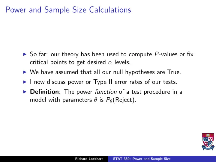
Power and Sample Size Calculations ◮ So far: our theory has been used to compute P -values or fix critical points to get desired α levels. ◮ We have assumed that all our null hypotheses are True. ◮ I now discuss power or Type II error rates of our tests. ◮ Definition : The power function of a test procedure in a model with parameters θ is P θ (Reject) . Richard Lockhart STAT 350: Power and Sample Size

t tests ◮ Consider a t -test of β k = 0. ◮ Test statistic is ˆ β k � MSE ( X T X ) − 1 kk ◮ Can be rewritten as the ratio � � � ˆ ( X T X ) − 1 β k / σ kk � [ SSE /σ 2 ] / ( n − p ) Richard Lockhart STAT 350: Power and Sample Size

◮ When null hypothesis that β k = 0 is true numerator is standard normal, the denominator is the square root of a chi-square divided by its degrees of freedom and the numerator and denominator are independent. ◮ When, in fact β k is not 0 the numerator is still normal and still has variance 1 but its mean is β k δ = . � ( X T X ) − 1 σ kk ◮ So define non-central t distribution as distribution of N ( δ, 1) � χ 2 ν /ν where the numerator and denominator are independent . ◮ The quantity δ is the noncentrality parameter . ◮ Table B.5 on page 1327 gives the probability that the absolute value of a non-central t exceeds a given level. Richard Lockhart STAT 350: Power and Sample Size

◮ If we take the level to be the critical point for a t test at some level α then the probability we look up is the corresponding power , ◮ That is, the probability of rejection. ◮ Notice power depends on two unknown quantities, β k and σ and on 1 quantity which is sometimes under the experimenter’s control (in a designed experiment) and sometimes not (as in an observational study.) ◮ Same idea applies to any linear statistic of the form a T ˆ β ◮ Get a non-central t distribution on the alternative. ◮ So, for example, if testing a T β = a 0 but in fact a T β = a 1 the non-centrality parameter is a 1 − a 0 δ = . � σ a T ( X T X ) − 1 a Richard Lockhart STAT 350: Power and Sample Size

Sample Size determination ◮ Before an experiment is run. ◮ Sometimes experiment is costly. ◮ So try to work out whether or not it is worth doing. ◮ Only do experiment if probabilities of Type I and II errors both reasonably low. ◮ Simplest case arises when you prespecify a level, say α = 0 . 05 and an acceptable probability of Type II error, β say 0.10. Richard Lockhart STAT 350: Power and Sample Size

◮ Then you need to specify ◮ The ratio β/σ : comes from physically motivated understanding of what value of β would be important to detect and from understanding of reasonable values for σ . ◮ How the design matrix would depend on the sample size. ◮ Easiest: fix some small set of say j values x 1 , . . . , x j ; then use each member of that set say m times so that the aggregate sample size is mj . ◮ This gives a non-centrality parameter of the form √ m β σ × � ( X T X ) − 1 kk ◮ The value n = mj influences both the row in table B.5 which should be used and the value of δ . ◮ If the solution is large, however, then all the rows in B.5 at the bottom of the table are very similar so that effectively only δ depends on n ; we can then solve for n . Richard Lockhart STAT 350: Power and Sample Size

Power for F tests ◮ Simplest example: regression through origin (no intercept). ◮ Model Y i = β 1 X i , 1 + · · · + β p X i , p + ǫ i ◮ Test β 1 = · · · = β p = 0 ◮ F statistic Y T ˆ Y T HY / p ˆ F = MSR Y / p MSE = = Y T ( I − H ) Y / ( n − p ) . ǫ T ˆ ˆ ǫ Suppose now that the null hypothesis is false. ◮ Substitute Y = X β + ǫ in F . ◮ Use HX = X (and so ( I − H ) X = 0). ◮ Denominator is ǫ T ( I − H ) ǫ n − p Richard Lockhart STAT 350: Power and Sample Size

◮ So: even when the null hypothesis is false the denominator divided by σ 2 has the distribution of a χ 2 on n − p degrees of freedom divided by its degrees of freedom. ◮ FACT: Numerator and denominator are independent of each other even when the null hypothesis is false. ◮ Numerator is ( ǫ + X β ) T H ( ǫ + X β ) p ◮ Divide by σ 2 and rewrite this as W T HW / p ◮ W = ( ǫ + X β ) /σ has a multivariate normal distribution with mean X β/σ = µ/σ and variance the identity matrix. Richard Lockhart STAT 350: Power and Sample Size

◮ FACT: If W is a MVN ( τ, I ) random vector and Q is idempotent with rank p then W T QW has a non-central χ 2 distribution with non-centrality parameter δ 2 = E ( W T QW ) − p = τ T Q τ and p degrees of freedom. ◮ This is the same distribution as that of ( Z 1 + δ ) 2 + Z 2 2 + · · · + Z 2 p where the Z i are iid standard normals. An ordinary χ 2 variable is called central and has δ = 0. ◮ FACT: If U and V are independent χ 2 variables with degrees of freedom ν 1 and ν 2 , V is central and U is non-central with non-centrality parameter δ 2 then U /ν 1 V /ν 2 is said to have a non-central F distribution with non-centrality parameter δ 2 and degrees of freedom ν 1 and ν 2 . Richard Lockhart STAT 350: Power and Sample Size

Power Calculations ◮ Table B 11 gives powers of F tests for various small numerator degrees of freedom and a range of denominator degrees of freedom ◮ Must use α = 0 . 05 or α = 0 . 01. ◮ In table φ is our δ/ √ p + 1 (that is, the square root of what I called the non-centrality parameter divided by the square root of 1 more than the numerator degrees of freedom.) Richard Lockhart STAT 350: Power and Sample Size

Sample size calculations ◮ Sometimes done with charts and sometimes with tables; see table B 12. ◮ This table depends on a quantity � ( p + 1) δ 2 ∆ σ = n To use the table you specify ◮ α (one of 0.2, 0.1, 0.05 or 0.01) ◮ Power (= 1 − β in notation of table)– must be one of 0.7, 0.8, 0.9 or 0.95 ◮ Non-centrality per data point, δ 2 / n . Then you look up n . ◮ Realistic specification of δ 2 / n difficult in practice. Richard Lockhart STAT 350: Power and Sample Size

Example: POWER of t test: plaster example ◮ Consider fitting the model Y i = β 0 + β 1 S i + β 2 F i + β 3 F 2 i + ǫ i ◮ Compute power of t test of β 3 = 0 for the alternative β 3 = − 0 . 004. ◮ This is roughly the fitted value. ◮ In practice, however, this value needs to be specified before collecting data so you just have to guess or use experience with previous related data sets or work out a value which would make a difference big enough to matter compared to the straight line.) ◮ Need to assume a value for σ . ◮ I take 2.5 – a nice round number near the fitted value. ◮ Again, in practice, you will have to make this number up in some reasonable way. Richard Lockhart STAT 350: Power and Sample Size

◮ Finally a t = (0 , 0 , 0 , 1) and a T ( X T X ) − 1 a has to be computed. ◮ For the design actually used this is 6 . 4 × 10 − 7 . Now δ is 2. ◮ The power of a two-sided t test at level 0.05 and with 18 − 4 = 14 degrees of freedom is 0.46 (from table B 5 page 1327). ◮ Take notice that you need to specify α , β 3 /σ (or even β 3 and σ ) and the design! Richard Lockhart STAT 350: Power and Sample Size

Sample size needed using t test: plaster example ◮ Now for the same assumed values of the parameters how many replicates of the basic design (using 9 combinations of sand and fibre contents) would I need to get a power of 0.95? ◮ The matrix X T X for m replicates of the design actually used is m times the same matrix for 1 replicate. ◮ This means that a T ( X T X ) − 1 a will be 1 / m times the same quantity for 1 replicate. ◮ Thus the value of δ for m replicates will be √ m times the value for our design, which was 2. ◮ With m replicates the degrees of freedom for the t -test will be 18 m − 4. Richard Lockhart STAT 350: Power and Sample Size

◮ We now need to find a value of m so that in the row in Table B 5 across from 18 m − 4 degrees of freedom and the column corresponding to δ = 2 √ m we find 0.95. ◮ To simplify we try just assuming that the solution m is quite large and use the last line of the table. ◮ We get δ between 3 and 4 – say about 3.75. ◮ Now set 2 √ m = 3 . 7 and solve to find m = 3 . 42 which would have to be rounded to 4 meaning a total sample size of 4 × 18 = 72. ◮ For this value of m the non-centrality parameter is actually 4 (not the target of 3.75 because of rounding) and the power is 0.98. ◮ Notice that for this value of m the degrees of freedom for error is 66 which is so far down the table that the powers are not much different from the ∞ line. Richard Lockhart STAT 350: Power and Sample Size

POWER of F test: SAND and FIBRE example ◮ Now consider the power of the test that all the higher order terms are 0 in the model Y i = β 0 + β 1 S i + β 2 F i + β 3 F 2 i + β 4 S 2 i + β 5 S i F i + ǫ i that is the power of the F test of β 3 = β 4 = β 5 = 0. ◮ Need to specify the non-centrality parameter for this F test. ◮ In general the noncentrality parameter for a F test based on ν 1 numerator degrees of freedom is given by E (Extra SS) /σ 2 − ν 1 . ◮ This quantity needs to be worked out algebraically for each separate case, however, some general points can be made. Richard Lockhart STAT 350: Power and Sample Size