SLIDE 1 ECO 305 — FALL 2003 — December 2
PORTFOLIO CHOICE One Riskless, One Risky Asset Safe asset: gross return rate R (1 plus interest rate) Risky asset: random gross return rate r Mean µ = E[r] > R, Variance σ2 = V[r] Initial wealth W0. If x in risky asset, final wealth W = (W0 − x) R + x r = R W0 + (r − R) x E[W] = W0 R + x (µ − R) V[W] = x2 σ2;
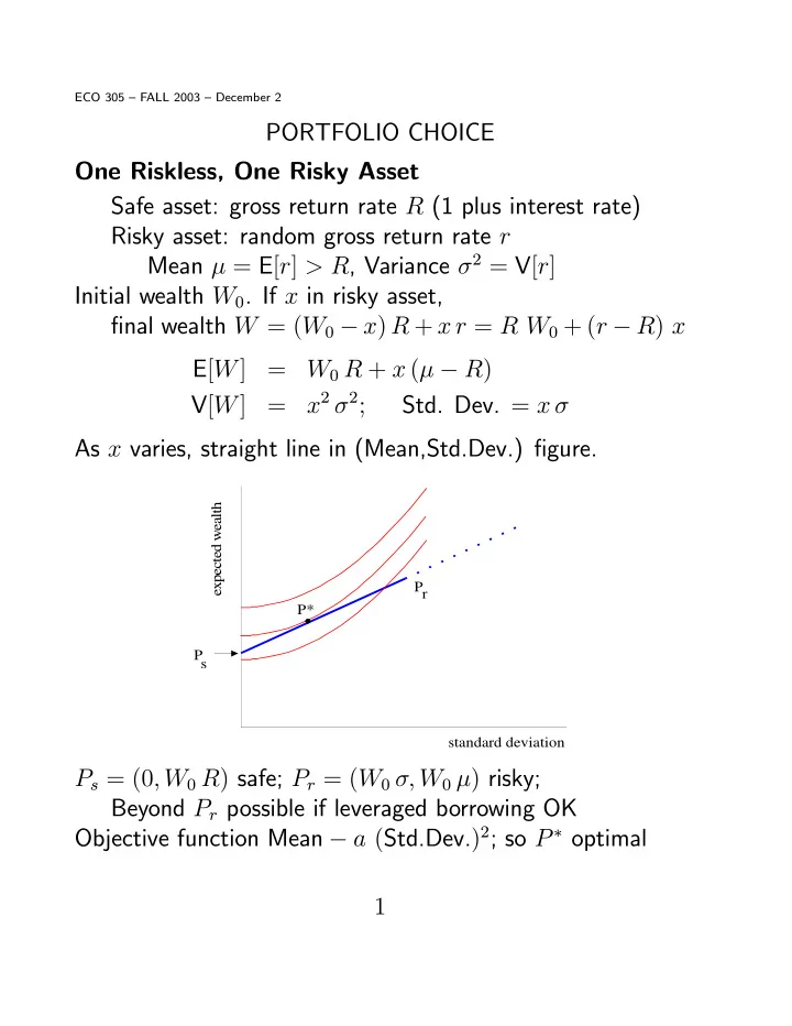
As x varies, straight line in (Mean,Std.Dev.) figure.
standard deviation expected wealth P P P* s r
Ps = (0, W0 R) safe; Pr = (W0 σ, W0 µ) risky; Beyond Pr possible if leveraged borrowing OK Objective function Mean − a (Std.Dev.)2; so P ∗ optimal 1
SLIDE 2
Two Risky Assets W0 = 1; Random gross return rates r1, r2 Means µ1 > µ2; Std. Devs. σ1, σ2, Correl. Coefft. ρ Portfolio (x, 1 − x). Final W = x r1 + (1 − x) r2 E[W] = x µ1 + (1 − x) µ2 = µ2 + x (µ1 − µ2) V[W] = x2 (σ1)2 + (1 − x)2 (σ2)2 + 2 x (1 − x) ρ σ1 σ2 = (σ2)2 − 2 x σ2 (σ2 − ρ σ1) + x2 [(σ1)2 − 2 ρ σ1 σ2 + (σ2)2]
standard deviation expected wealth P P P P* m 1 2
Diversification can reduce variance if ρ < min [σ1/σ2, σ2/σ1] P1, P2 points for the two individual assets Pm minimum-variance portfolio Portion P2 Pm dominated; Pm P1 efficient frontier Continuation past P1 if short sales of 2 OK Optimum P ∗ when preferences as shown 2
SLIDE 3 One Riskless, Two Risky Assets First combine two riskies; then mix with riskless
standard deviation expected wealth P P P P P P P* m r F 1 2 Ph s
This gets all points like Ph on all lines like Ps Pr Efficient frontier Ps PF tangential to risky combination curve Then along curve segment PF P1 if no leveraged borrowing; continue straight line Ps PF if leveraged borrowing OK With preferences as shown, optimum P ∗ mixes safe asset with particular risky combination PF “Mutual fund” PF is the same for all investors regardless of risk-aversion (so long as optimum in Ps PF) Even less risk-averse people may go beyond PF including corner solution at P1
- r tangency past P1 if can sell 2 short to buy more 1
3
SLIDE 4
CAPITAL ASSET PRICING MODEL Individual investors take the rates of return as given but these must be determined in equilibrium Add supply side — firms issue equities Take production, profit-max as exogenous Two firms, profits Π1 and Π2. Means E[Π1], E[Π2]; Variances V[Π1], V[Π2]; Covariance Cov[Π1, Π2] Safe asset (government bond) sure gross return rate R Market values of firms F1, F2; to be solved for (endogenous) (Random) rates of return r1 = Π1/F1 and r2 = Π2/F2, and for whole market, rm = (Π1 + Π2)/(F1 + F2) After a lot of algebra, important results: (1) E[r1] − R = Cov[r1, rm] V[rm] { E[rm] − R } Risk premium on firm-1 stock depends on its systematic risk (correlation with whole market) only, not idiosyncratic risk (part uncorrelated with market) Coefficient is beta of firm-1 stock (2) F1 = E[Π1] − A Cov[Π1, Π1 + Π2] R where A is the market’s aggregate risk-aversion (usually small) Value of firm = present value of its profits adjusted for systematic risk, and discounted at riskless rate of interest 4
SLIDE 5 ROCKET-SCIENCE FINANCE Equity, debt etc - complex pattern of payoffs in different scenarios: vector S = (S1, S2, . . .) Owning security S is full equivalent to
- wning portfolio of Arrow-Debreu securities (ADS):
S1 of ADS1, S2 of ADS2, . . . In equilibrium, no “riskless arbitrage” profit available So relation bet. price PS of S and ADS prices pi: PS = S1 p1 + S2 p2 + . . . Converse example: Two scenarios, two firms’s shares payoff MicTel (M1, M2), BioWiz (B1, B2). If XM of MicTel + XB of BioWiz ≡ 1 of ADS1, XM M1 + XB B1 = 1, XM M2 + XB B2 = 0 XM = B2 M1 B2 − B1 M2 , XB = −M2 M1 B2 − B1 M2 One of these may be negative: need short sales 5
SLIDE 6
ADS’s can be “constructed” from available securities Then no-arbitrage-in-equilibrium condition: P1 = XM PMicTel + XB PBioWiz Similarly P2. So the “constructed” ADS’s can be priced. Every financial asset is defined by its vector of payoffs in all scenarios. Therefore it can be priced using these prices of all ADS’s (“pricing kernel”) Examples — options and other derivatives General idea: Markets for risks are complete, and achieve Pareto-efficient allocation of risks if enough securities exist that their payoff vectors span the space of wealths in all scenarios “Rocket-science finance” extends this idea to infinite-dimensional spaces of scenarios If sequence of periods, need enough markets to span the scenarios one-period ahead, and then rebalance portfolio by trade (dynamic hedging) Finance = General equilibrium + Linear algebra ! Recent research: (1) Asset pricing with incomplete markets (2) Strategic trading with / against asymmetric info 6