Polynomial Functions In Factored Form MHF4U: Advanced Functions - - PDF document

p o l y n o m i a l f u n c t i o n s

MHF4U: Advanced Functions

Equations and Graphs of Polynomial Functions

• J. Garvin

Slide 1/18

p o l y n o m i a l f u n c t i o n s

Polynomial Functions In Factored Form

Polynomials are generally written in standard form, such as f (x) = x3 + 4x2 + x − 6. A more useful way to write a polynomial function’s equation is to use factored form, such as f (x) = (x − 1)(x + 2)(x + 3). Each factor corresponds to an x-intercept of the function.

Factored Form of a Polynomial Function

An equation of a polynomial function is in factored form if it is written as f (x) = a(x − r1)(x − r2) . . . (x − rn), where (x − rk) is a factor corresponding to x-intercept rk. Note that it is not always possible to express a polynomial function using factored form.

• J. Garvin — Equations and Graphs of Polynomial Functions

Slide 2/18

p o l y n o m i a l f u n c t i o n s

Polynomial Functions In Factored Form

Example

Identify the factors, and x-intercepts, of the polynomial function f (x) = −2x(x + 5)(x − 3). f (x) has three factors: x, x + 5 and x − 3. These factors correspond to x-intercepts 0, −5 and 3.

• J. Garvin — Equations and Graphs of Polynomial Functions

Slide 3/18

p o l y n o m i a l f u n c t i o n s

Order of a Factor

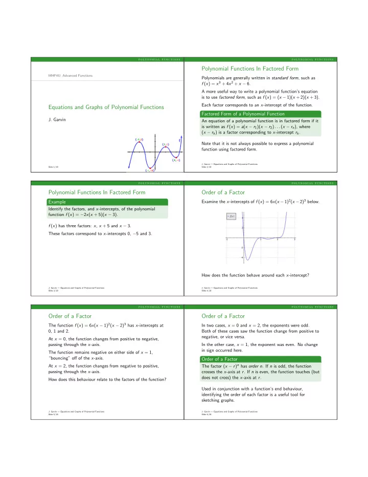
Examine the x-intercepts of f (x) = 6x(x − 1)2(x − 2)3 below. How does the function behave around each x-intercept?

• J. Garvin — Equations and Graphs of Polynomial Functions

Slide 4/18

p o l y n o m i a l f u n c t i o n s

Order of a Factor

The function f (x) = 6x(x − 1)2(x − 2)3 has x-intercepts at 0, 1 and 2. At x = 0, the function changes from positive to negative, passing through the x-axis. The function remains negative on either side of x = 1, “bouncing” off of the x-axis. At x = 2, the function changes from negative to positive, passing through the x-axis. How does this behaviour relate to the factors of the function?

• J. Garvin — Equations and Graphs of Polynomial Functions

Slide 5/18

p o l y n o m i a l f u n c t i o n s

Order of a Factor

In two cases, x = 0 and x = 2, the exponents were odd. Both of these cases saw the function change from positive to negative, or vice versa. In the other case, x = 1, the exponent was even. No change in sign occurred here.

Order of a Factor

The factor (x − r)n has order n. If n is odd, the function crosses the x-axis at r. If n is even, the function touches (but does not cross) the x-axis at r. Used in conjunction with a function’s end behaviour, identifying the order of each factor is a useful tool for sketching graphs.

• J. Garvin — Equations and Graphs of Polynomial Functions

Slide 6/18

p o l y n o m i a l f u n c t i o n s

Graphs of Polynomial Functions

Example

Sketch a graph of f (x) = (x + 3)2(x − 1). f (x) has two distinct x-intercepts, at x = −3 and x = 1. Another way to write the equation is f (x) = (x + 3)(x + 3)(x − 1). Multiplying all terms containing x, we obtain x3, so f (x) has degree 3 (cubic). The leading coefficient is positive, so f (x) has Q3-Q1 end

• behaviour. Therefore, f (x) is negative as x → −∞.

Moving from left to right, the first x-intercept is at x = −3, where it has order 2. Thus, the function touches the x-axis at x = −3, but stays negative beyond it. The next x-intercept is at x = 1, where it has order 1. f (x) changes from negative to positive at x = 1.

• J. Garvin — Equations and Graphs of Polynomial Functions

Slide 7/18

p o l y n o m i a l f u n c t i o n s

Order of a Factor

One final piece point is the y-intercept, which can be found by multiplying all of the constant terms and the leading coefficient. In this case, the y-intercept is (3)(3)(−1) = −9.

• J. Garvin — Equations and Graphs of Polynomial Functions

Slide 8/18

p o l y n o m i a l f u n c t i o n s

Graphs of Polynomial Functions

Example

Sketch a graph of f (x) = −2x(x + 1)(x − 2)2. f (x) has three distinct x-intercepts, at x = −1, x = 0 and x = 2. f (x) is a quartic function, with degree 4. The leading coefficient is negative, so f (x) has Q3-Q4 end

• behaviour. f (x) is negative as x → −∞.

From left to right, f (x) changes from negative to positive at x = −1, changes from positive to negative at x = 0, and touches the x-axis at x = 2. The y-intercept is −2(0)(1)(−2)(−2) = 0.

• J. Garvin — Equations and Graphs of Polynomial Functions

Slide 9/18

p o l y n o m i a l f u n c t i o n s

Graphs of Polynomial Functions

• J. Garvin — Equations and Graphs of Polynomial Functions

Slide 10/18

p o l y n o m i a l f u n c t i o n s

Graphs of Polynomial Functions

Example

Given the graph of f (x) below, state the minimum possible degree, sign of the leading coefficient, factors, x-intercepts and intervals where the function is positive or negative.

• J. Garvin — Equations and Graphs of Polynomial Functions

Slide 11/18

p o l y n o m i a l f u n c t i o n s

Graphs of Polynomial Functions

f (x) has Q2-Q4 end behaviour, so the degree must be odd and the leading coefficient is negative. There are x-intercepts at x = −3 (even order), x = 0 (odd

• rder) and x = 2 (even order), so the minimum degree is 5.

This is confirmed by the fact that there are 4 local minimums and maximums. f (x) is positive on the intervals (−∞, −3) ∪ (−3, 0). Since zero is neither positive nor negative, it is not included in the interval. f (x) is negative on the intervals (0, 2) ∪ (2, ∞).

• J. Garvin — Equations and Graphs of Polynomial Functions

Slide 12/18

p o l y n o m i a l f u n c t i o n s

Symmetry

Recall that an even function is symmetric in the f (x)-axis. Any function that is symmetric in the f (x)-axis has the property that f (x) = f (−x).

• J. Garvin — Equations and Graphs of Polynomial Functions

Slide 13/18

p o l y n o m i a l f u n c t i o n s

Symmetry

An odd function is point-symmetric about the origin. Any function that has point symmetry about the origin has the property that f (−x) = −f (x).

• J. Garvin — Equations and Graphs of Polynomial Functions

Slide 14/18

p o l y n o m i a l f u n c t i o n s

Symmetry

Example

Verify algebraically that f (x) = 2x4 + 3x2 − 1 is symmetric in the f (x)-axis. f (−x) = 2(−x)4 + 3(−x)2 − 1 = 2x4 + 3x2 − 1 = f (x) Therefore, f (x) is symmetric in the f (x)-axis. It is an even function.

• J. Garvin — Equations and Graphs of Polynomial Functions

Slide 15/18

p o l y n o m i a l f u n c t i o n s

Symmetry

Example

Algebraically classify f (x) = 2x3 + x2 − 5x as even, odd or neither. Test if f (x) is even first. f (−x) = 2(−x)3 + (−x)2 − 5(−x) = −2x3 + x2 + 5x = f (x) Therefore, f (x) is not even.

• J. Garvin — Equations and Graphs of Polynomial Functions

Slide 16/18

p o l y n o m i a l f u n c t i o n s

Symmetry

Test if f (x) is odd next. f (−x) = −2x3 + x2 + 5x − f (x) = −(2x3 + x2 − 5x) = −2x3 − x2 + 5x f (−x) = −f (x) Therefore, f (x) is not odd either.

• J. Garvin — Equations and Graphs of Polynomial Functions

Slide 17/18

p o l y n o m i a l f u n c t i o n s

Questions?

• J. Garvin — Equations and Graphs of Polynomial Functions

Slide 18/18