PERT and Monte Carlo Simulation for Project Scheduling Until now we - PDF document

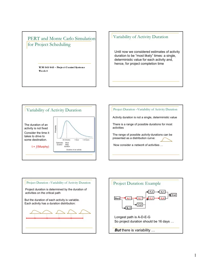
Variability of Activity Duration PERT and Monte Carlo Simulation for Project Scheduling Until now we considered estimates of activity duration to be “most likely” times: a single, deterministic value for each activity and, hence, for project completion time T CM 545/ 645 – Pr oje c t Contr ol Syste ms We e k 3 Variability of Activity Duration Project Duration –Variability of Activity Duration Activity duration is not a single, deterministic value There is a range of possible durations for most The duration of an activities activity is not fixed Consider the time it The range of possible activity durations can be takes to drive to presented as a distribution curve: some destination. Now consider a network of activities … t = ƒ(Murphy) Project Duration –Variability of Activity Duration Project Duration: Example Project duration is determined by the duration of activities on the critical path But the duration of each activity is variable. Each activity has a duration distribution: Longest path is A-D-E-G So project duration should be 16 days … But there is variability … 1

Project Duration The PERT Technique (Program Evaluation & Review Technique)  In reality, actual activity times will vary, hence so PERT: will project completion time. Program Evaluation  Might say that, e.g., project will be completed in and Review 16 days, but also acknowledge it will likely be completed earlier or later than that. Technique The PERT technique addresses variability of the duration of activities on the critical path PERT (cont’d) PERT history  PERT treats completion times as probabilistic Was developed in the 1950s for (stochastic) events the USA Polaris Missile-submarine  PERT deals with uncertainty in projects, and to program estimate project duration when activity times are  USA Naval Office of Special Projects hard to estimate  Lockheed Corporation  PERT answers questions e.g. (now Lockheed-Martin)  Booz, Allen, Hamilton Corporation  What is probability of completing project within 20 days?  If we want a 95% level of confidence, what should the project duration be? Where did PERT originate? PERT Technique (Cont’d) PERT Technique (Cont’d) Pessimistic duration b : Assume duration of every activity is range of times, represented by a probability distribution Exclude highly unlikely events e.g. Distribution is based upon Earthquakes  three estimates for each Labor strikes activity:  a = optimistic m = most likely  Definite cut-off point for b b = pessimistic a m b? What should the pessimistic duration be? 2

PERT Technique (Cont’d) PERT Technique (Cont’d) Now, given the a, b and m estimates, for Definite cut-off point for the pessimistic value every activity compute expected time t e Where a = optimistic m = most likely b = pessimistic t e is the expected duration for an activity (50% chance of activity completed by t e ) The sum of t e values of activities on the critical path = T e e =  t e Mean Project duration = T CP (50% chance of project completed by T e ) PERT Technique (Cont’d) PERT Technique (Cont’d) Also, given the a, b and m estimates, for These formulas are based on the assumption that every activity compute the standard each activity duration is a Beta distribution (not deviation,  Normal distribution) Beta Distribution:  Could be skewed (not symmetrical)  Definite cut-off points  A single peak a m b Where “V” is the variance. PERT Technique (Cont’d) PERT Technique (Cont’d) Step 2: Step 1: Identify the critical path, based on t e values ( not m-values)  For each activity calculate the t e value ( a + 4 m + b )/6  Everywhere in network, insert expected time, t e CP is A-D-E-G, which indicates expected project completion time, T e = 16 days (50% chance) What is probability that project will be completed in 20 days? Assume times shown are t e, 3

PERT Technique (Cont’d) PERT Technique (Cont’d) Step 3: Step 3 (Cont’d) Consider the summative distribution of all Consider the summative distribution of all activities on the critical path activities on the critical path T e = expected project Assume distribution of project completion is normal, completion date =16 days not skewed  50% probability of duration (justified by the Central Limit Theorem – discussed later) being less than 16 days, 50% 50% (and 50% probability of it exceeding 16 days) PERT Technique (Cont’d) PERT Technique (Cont’d) Step 3 (Cont’d): Consider the summative distribution of all activities on the critical path T e T s To determine the probability of T s = the project duration under consideration (time of interest, finishing the project within 20 i.e. 20 days) days, compute the area to left T e = the expected project duration of 20 on distribution, P (x ≤ 20) Z = number of standard deviations that T s is from the mean ? z = ( T s – T e ) /  project duration σ = standard deviation for project (found by summing the variance of each activity along the critical path and then taking the square root of the total) Technique (cont’d) Technique (cont’d) Step 4: Compute T e ,  , and variance for the critical path Assume the following values are given: CP t e   2 = V =variance T e T s A 1 1 1  e = 16 T s =20 D 7 2 4 E 2 1 1 T e = expected project duration = Σ t e G 6 1 1 Total for CP: 16 = T e 7 = V T s = project completion time of interest V project = ∑ V CP = ∑  2 = 7 (see later why we add up variances) 4

Technique (cont’d) Technique (cont’d) P (z ≤ 1.52) = 0.93 Thus, V P = ∑  = 7, so  =  7 (approximately 93%. As estimates are used, higher accuracy does not make sense) Compute z–value T e T s  e = 16 T s =20 For project duration of 20 days: T s - ∑ t e 20 - 16 = = 1.52 Z =  p √ 7 Hence, conclude that there is a 93% probability that the project will be completed in 20 days or less Summary: The Role of PERT Interpretation On its own PERT does not reduce project duration  Now the question is: How confident are However, it does the following: we in the 93% estimate? How much do 1. Given a network with estimates a, m, and b as well as a you trust that estimate? value for project duration, it provides a probability figure for finishing on time  93% is high percentage. So, can we be 2. Alternatively, given a network with estimates a, m, and b as well as a desired level of confidence (probability figure, very confident that project will be finished say 99%), it can calculate a project duration that in less than 20 days? corresponds with the level of confidence 3. It provides insight in the effect of variability of activity duration on the critical path Interpretation PERT only considers the critical path There are often paths that are “near critical” Answer: 1. Confidence in estimates a, m, and b  If estimates are based upon experience backed by historical data, maybe we can believe the 93% estimate  If a, m, and b are guesses, be careful! If any of these estimates are substantially incorrect, the computed % will be meaningless 2. The method only considers the critical path and is misleading when near-critical paths could become critical 5

Shortcoming: Merge-point bias PERT only considers the critical path PERT only considers the critical path and is misleading when near-critical paths could become critical Merge-point bias: Five paths merging, each with 50% chance of being on time Probability of project finishing on time = (0.5 5  .03 or 3%) Two paths merging, each 50% chance of being on time 25% chance of finishing on time (or early) c.a. 3% chance of finishing on time Non-critical paths and merge-point bias Non-critical paths and merge-point bias Merge-point bias addressed by Monte-Carlo simulation The problem of near-critical paths that could of the network become critical and merge-point bias can be addressed by Monte-Carlo simulation of the entire network Times for project critical and non-critical activities are randomly selected from probability distributions (based on random numbers) The critical path is computed from these times The procedure is repeated many times to generate a distribution diagram for duration of the project We will use the statistical analysis software package called @Risk to study Monte Carlo simulations of project schedules. Other Shortcomings of PERT Risk of Adding Up Most Likely Values  Assumes that a successor will start immediately In practice many managers simply add up when predecessors completed, also when an activity durations on the critical path and activity is completed earlier than indicated on the are not aware of the risk of doing so schedule (They also add up most likely cost figures)  PERT technique can provide false confidence Let’s look at the risk of this deterministic  Expecting high probability of project completion, approach (consider only the critical path of managers let their guard down! (PERT does not a project) take behavioral aspects into account) 6