Perceptron Learning Algorithm Matthieu R. Bloch 1 A bit of - - PDF document

ECE 6254 - Spring 2020 - Lecture 9 v1.1 - revised February 4, 2020

Perceptron Learning Algorithm

Matthieu R. Bloch

1 A bit of geometry Definition 1.1. Dataset {xi, yi}N

i=1 is linearly separable if there exists w ∈ Rd and b ∈ R such that

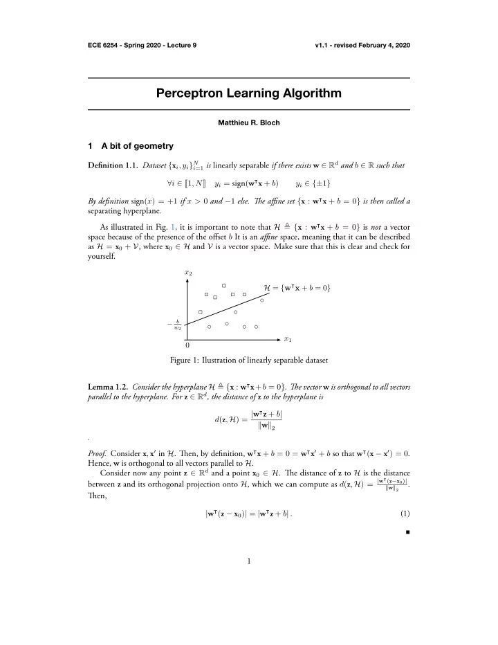
∀i ∈ 1, N yi = sign(w⊺x + b) yi ∈ {±1} By definition sign(x) = +1 if x > 0 and −1 else. Tie affine set {x : w⊺x + b = 0} is then called a separating hyperplane. As illustrated in Fig. 1, it is important to note that H ≜ {x : w⊺x + b = 0} is not a vector space because of the presence of the offset b It is an affine space, meaning that it can be described as H = x0 + V, where x0 ∈ H and V is a vector space. Make sure that this is clear and check for yourself. x1 x2 H = {w⊺x + b = 0} − b

w2

Figure 1: Ilustration of linearly separable dataset Lemma 1.2. Consider the hyperplane H ≜ {x : w⊺x+b = 0}. Tie vector w is orthogonal to all vectors parallel to the hyperplane. For z ∈ Rd, the distance of z to the hyperplane is d(z, H) = |w⊺z + b| ∥w∥2 .

• Proof. Consider x, x′ in H. Tien, by definition, w⊺x + b = 0 = w⊺x′ + b so that w⊺(x − x′) = 0.

Hence, w is orthogonal to all vectors parallel to H. Consider now any point z ∈ Rd and a point x0 ∈ H. Tie distance of z to H is the distance between z and its orthogonal projection onto H, which we can compute as d(z, H) = |w⊺(z−x0)|

∥w∥2

. Tien, |w⊺(z − x0)| = |w⊺z + b| . (1)

■

1

ECE 6254 - Spring 2020 - Lecture 9 v1.1 - revised February 4, 2020

2 The Perceptron Learning Algorithm Tie Perceptron Learning Algorithm (PLA) was proposed by Rosenblatt to identify a separating hyperplane in a linearly separarable dataset {(xi, yi)}N

i=1 if it exist. We assume that every vector

x ∈ Rd+1 with x0 = 1, so that we can use the shorthand θ⊺x = 0 to describe a affine hyperplane. Tie principle of the algorithm is the following.

• 1. Start from a guess θ(0).
• 2. For j ⩾ 1, iterate over the data points (in any order) and update

θ(j+1) = { θ(j) + yixi if yi ̸= sign ( θ(j)⊺xi ) θ(j) else (2) Geometric view of PLA Tie effect of the PLA update is illustrated in Fig. 2. Note that the update

• f θ(j+1) not only changes the overall hyperplane, and not just the associated vector space. Tiis is

best seen in Fig. 2, where the offset changes and not just the slope of the separator.

• ✐

Figure 2: PLA update Gradient descent view of PLA Consider a loss function called the “perceptron loss” defined as ℓ(θ) ≜

N

∑

i=1

max(0, −yiθ⊺xi). (3) Intuitively, the loss penalizes misclassified points (according to θ) with a penalty proportional to how badly they are misclassified. Setting ℓi(θ) ≜ max(0, −yiθ⊺xi), we have ∇ℓi(θ) =      0 if yiθ⊺xi > 0 −yixi if yiθ⊺xi < 0 [0, 1] × −yixi if θ⊺xi = 0 (4) Tie case of equality θ⊺xi = 0 corresponds to the point where the loss function ℓi(θ) is not differ-

• entiable. In such case, we have to use a subgradient of ℓi at θ, which is any vector v such that for all

θ′, ℓi(θ) − ℓi(θ′) ⩾ v⊺(θ − θ′). A subgradient is not unique and the set of subgradients is usually denoted ∂ℓi(θ). Let us now apply a stochastic gradient descent algorithm with a step size of 1 to the loss function. We obtain 2

ECE 6254 - Spring 2020 - Lecture 9 v1.1 - revised February 4, 2020

• 1. Start from a guess θ(0).
• 2. For j ⩾ 1, iterate over the data points (in any order) and update

θ(j+1) = θ(j) − ∇ℓi(θ) =      θ(j) + yixi if − yiθ(j)⊺xi > 0 θ(j) if − yiθ(j)⊺xi < 0 θ(j) − v where v ∈ ∂ℓi(θ) if θ⊺xi = 0 (5) Note that (5) is almost identical to (2). Tie PLA udpate rule is essentially a stochastic gradient descent that treats the case of subgradients with its own rule. Tieorem 2.1. Consider a linearly separable data set {(xi, yi)}N

i=1. Tie number of updates made by the

PLA because of classification errors is bounded and the PLA eventually identifies a separating hyperplane. 3 To go further A simple and accessible review of gradient descent techniques can be found in [1]. Tie original proposal of the PLA is in [2]. Introductory treatments of the PLA are found in [3, Section 4.5] and [4, Section 8.5.4]. References [1] S. Ruder, “An overview of gradient descent optimization algorithms,” arXiv preprint, Jun. 2017. [2] F. Rosenblatt, “Tie perceptron: A probabilistic model for information storage and organization in the brain,” Psychological Review, vol. 65, no. 6, pp. 386–408, 1958. [3] T. Hastie, R. Tibshirani, and J. H. Friedman, Tie Elements of Statistical Learning: Data Mining, Inference, and Prediction, ser. Springer series in statistics. Springer, 2009. [4] K. P . Murphy, Machine Learning: A Probabilistic Perspective. MIT Press, 2012. 3