Perceptron Homework Assume a 3 input perceptron plus bias (it - PowerPoint PPT Presentation

Perceptron Homework Assume a 3 input perceptron plus bias (it outputs 1 if net > 0, else 0) l Assume a learning rate c of 1 and initial weights all 1: Δ w i = c ( t – z) x i l Show weights after each pattern for just one epoch l Training set 1 0 1 -> 0 l 1 1 0 -> 0 1 0 1 -> 1 0 1 1 -> 1 Pattern Target Weight Vector Net Output Δ W 1 0 1 1 0 1 1 1 1 3 1 -1 0 -1 -1 1 1 0 1 0 0 1 0 0 1 1 -1-1 0 -1 1 0 1 1 1 -1 0 0 -1 -2 0 1 0 1 1 0 1 1 1 1 0 0 1 0 1 1 0 0 0 0 0 0 1 0 CS 478 - Perceptrons 1

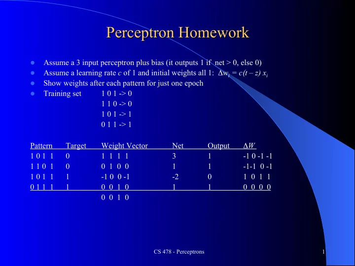
Quadric Machine Homework Assume a 2 input perceptron expanded to be a quadric perceptron (it outputs 1 if l net > 0, else 0). Note that with binary inputs of -1, 1, that x 2 and y 2 would always be 1 and thus do not add info and are not needed (they would just act like to more bias weights) Assume a learning rate c of .4 and initial weights all 0: Δ w i = c ( t – z) x i l Show weights after each pattern for one epoch with the following non-linearly l separable training set. Has it learned to solve the problem after just one epoch? l Which of the quadric features are actually needed to solve this training set? l x y Target -1 -1 0 -1 1 1 1 -1 1 1 1 0 CS 478 - Regression 2

Quadric Machine Homework l wx represents the weight for feature x l Assume a 2 input perceptron expanded to be a quadric perceptron (it outputs 1 if net > 0, else 0) l Assume a learning rate c of .4 and initial weights all 0: Δ w i = c ( t – z) x i l Show weights after each pattern for one epoch with the following non- linearly separable training set. l Has it learned to solve the problem after just one epoch? l Which of the quadric features are actually needed to solve this training set? x y xy wx wy wxy bias Δ wx Δ wx Δ wxy Δ bias net Target Output -1 -1 1 0 0 0 0 0 0 0 0 0 0 0 -1 1 -1 0 0 0 0 -.4 .4 -.4 .4 0 1 0 1 -1 -1 -.4 .4 -.4 .4 .4 -.4 -.4 .4 0 1 0 1 1 1 0 0 -.8 .8 0 0 0 0 -.8 0 0 0 0 -.8 .8 CS 478 - Regression 3

Quadric Machine Homework l wx represents the weight for feature x l Assume a 2 input perceptron expanded to be a quadric perceptron (it outputs 1 if net > 0, else 0) l Assume a learning rate c of .4 and initial weights all 0: Δ w i = c ( t – z) x i l Show weights after each pattern for one epoch with the following non- linearly separable training set. l Has it learned to solve the problem after just one epoch? - Yes l Which of the quadric features are actually needed to solve this training set? – Really only needs feature xy . x y xy wx wy wxy bias Δ wx Δ wx Δ wxy Δ bias net Target Output -1 -1 1 0 0 0 0 0 0 0 0 0 0 0 -1 1 -1 0 0 0 0 -.4 .4 -.4 .4 0 1 0 1 -1 -1 -.4 .4 -.4 .4 .4 -.4 -.4 .4 0 1 0 1 1 1 0 0 -.8 .8 0 0 0 0 -.8 0 0 0 0 -.8 .8 CS 478 - Regression 4

Linear Regression Homework l Assume we start with all weights as 0 (don’t forget the bias) l What are the new weights after one iteration through the following training set using the delta rule with a learning rate of .2 x y Target .3 .8 .7 -.3 1.6 -.1 .9 0 1.3 CS 478 - Homework 5

Linear Regression Homework Δ w i = c ( t − net ) x i l Assume we start with all weights as 0 (don’t forget the bias) l What are the new weights after one iteration through the following training set using the delta rule with a learning rate c = .2 x y Target Net w 1 w 2 Bias 0 0 0 0 + .2(.7 – 0).3 = .042 .3 .8 .7 0 .042 .112 .140 -.3 1.6 -.1 .307 .066 -.018 .059 .9 0 1.3 .118 .279 -.018 .295 CS 478 - Homework 6

Logistic Regression Homework l You don’t actually have to come up with the weights for this one, though you could quickly by using the closed form linear regression approach l Sketch each step you would need to learn the weights for the following data set using logistic regression l Sketch how you would generalize the probability of a heart attack given a new input heart rate of 60 Heart Rate Heart Attack 50 Y 50 N 50 N 50 N 70 N 70 Y 90 Y 90 Y 90 N 90 Y 90 Y CS 478 - Homework 7

Logistic Regression Homework Calculate probabilities or odds for each input value 1. Calculate the log odds 2. Do linear regression on these 3 points to get the logit line 3. To find the probability of a heart attack given a new input heart 4. rate of 60, just calculate p = e logit(60) /(1+e logit(60) ) where logit(60) is the value on the logit line for 60 Heart Rate Heart Attack Heart Rate Heart Total Probability: Odds: Log Attacks Patients # attacks/ p/ (1- p ) = Odds: 50 Y Total # attacks/ 50 N Patients # not ln(Odds) 50 N 50 N 50 1 4 .25 .33 -1.11 70 N 70 1 2 .5 1 0 70 Y 90 Y 90 4 5 .8 4 1.39 90 Y 90 N 90 Y 90 Y CS 478 - Homework 8

BP-1) A 2-2-1 backpropagation model has initial weights as shown. Work through one cycle of learning for the f ollowing pattern(s). Assume 0 momentum and a learning constant of 1. Round calculations to 3 significant digits to the right of the decimal. Give values for all nodes and links for activation, output, error signal, weight delta, and final weights. Nodes 4, 5, 6, and 7 are just input nodes and do not have a sigmoidal output. For each node calculate the following (show necessary equati on for each). Hint: Calculate bottom-top-bottom. a = o = = w = w = 1 4 2 3 +1 7 5 6 +1 a) All weights initially 1.0 Training Patterns 1) 0 0 -> 1 2) 0 1 -> 0 CS 478 – Backpropagation 9

BP-1) net2 = wi xi = (1*0 + 1*0 + 1*1) = 1 net3 = 1 o2 = 1/(1+e-net) = 1/(1+e-1) = 1/(1+.368) = .731 o3 = .731 o4 = 1 net1 = (1*.731 + 1*.731 + 1) = 2.462 o1 = 1/(1+e-2.462)= .921 1 = (t1 - o1) o1 (1 - o1) = (1 - .921) .921 (1 - .921) = .00575 w21 = j oi = 1 o2 = 1 * .00575 * .731 = .00420 w31 = 1 * .00575 * .731 = .00420 w41 = 1 * .00575 * 1 = .00575 2 = oj (1 - oj) k wjk = o2 (1 - o2) 1 w21 = .731 (1 - .731) (.00575 * 1) = .00113 3 = .00113 w52 = j oi = 2 o5 = 1 * .00113 * 0 = 0 w62 = 0 w72 = 1 * .00113 * 1 = .00113 w53 = 0 w63 = 0 w73 = 1 * .00113 * 1 = .00113 1 4 2 3 +1 7 5 6 CS 478 – Backpropagation 10 +1

Second pass for 0 1 -> 0 Modified Weights: w21 = 1.0042 w31 = 1.0042 w41 = 1.00575 w52 = 1 w62 = 1 w72 = 1.00113 w53 = 1 w63 = 1 w73 = 1.00113 net2 = wi xi = (1*0 + 1*1 + 1*1.00113) = 2.00113 net3 = 2.00113 o2 = 1/(1+e-net) = 1/(1+e-2.00113) = .881 o3 = .881 o4 = 1 net1 = (1.0042*.881 + 1.0042*.881 + 1.00575*1) = 2.775 o1 = 1/(1+e-2.775)= .941 1 = (t1 - o1) o1 (1 - o1) = (0 - .941) .941 (1 - .941) = -.0522 w21 = j oi = 1 o2 = 1 * -.0522 * .881 = -.0460 w31 = 1 * -.0522 * .881 = -.0460 w41 = 1 * -.0522 * 1 = -.0522 2 = oj (1 - oj) k wjk = o2 (1 - o2) 1 w21 = .881 (1 - .881) (-.0522 * 1.0042) = -.00547 3 = -.00547 w52 = j oi = 2 o5 = 1 * -.00547* 0 = 0 w62 = 1 * (-.00547) * 1 = -.00547 w72 = 1 * (-.00547) * 1 = -.00547 w53 = 0 w63 = -.00547 w73 = 1 * (-.00547) * 1 = -.00547 w21 = 1.0042 - .0460 = .958 w31 = 1.0042 - .0460 = .958 w41 = 1.00575 - .0522 = .954 w52 = 1 + 0 = 1 w62 = 1 - .00547 = .995 w72 = 1.00113 - .00547 = .996 w53 = 1 + 0 = 1 w63 = 1 - .00547 = .995 CS 478 – Backpropagation 11 w73 = 1.00113 - .00547 = .996

Terms PCA Homework m 5 Number of instances in data set n 2 Number of input features p 1 Final number of principal components chosen • Use PCA on the given data set to get a transformed data set with just one feature (the first principal Original Data component (PC)). Show your work along the way. x y • Show what % of the total information is contained in p1 .2 -.3 the 1 st PC. p2 -1.1 2 • Do not use a PCA package to do it. You need to go p3 1 -2.2 p4 .5 -1 through the steps yourself, or program it yourself. p5 -.6 1 • You may use a spreadsheet, Matlab, etc. to do the mean 0 -.1 arithmetic for you. • You may use any web tool or Matlab to calculate the eigenvectors from the covariance matrix. CS 478 - Homework 12

Terms PCA Homework m 5 Number of instances in data set n 2 Number of input features p 1 Final number of principal components chosen Original Data Zero Centered Data Covariance Matrix EigenVectors x y x y x y x y Eigenvalue p1 .2 -.3 p1 .2 -.2 .715 -1.39 -.456 -.890 3.431 p2 -1.1 2 p2 -1.1 2.1 -1.39 2.72 -.890 -.456 .0037 p3 1 -2.2 p3 1 -2.1 % total info in 1 st principal component p4 .5 -1 p4 .5 -.9 3.431/(3.431 + . 0037) = 99.89% p5 -.6 1 p5 -.6 1.1 mean 0 -.1 mean 0 0 A × B New Data Set Matrix A – p × n Matrix B = Transposed zero centered 1 st PC Training Set x y p1 .0870 p1 p2 p3 p4 p5 1 st PC -.456 -.890 p2 -1.368 x .2 -1.1 1 .5 -.6 p3 1.414 y -.2 2.1 -2.1 -.9 1.1 p4 0.573 p5 -0.710 CS 478 - Homework 13