
SLIDE 1
Peer-to-peer overlay networks
Issue Large-scale distributed computer systems are spread across the Internet, yet their constituents need to communicate directly with each other ) organize the system in an overlay network. Overlay network Collection of peers, where each peer maintains a partial view
- f the system. View is nothing but a list of other peers with
whom communication connections can be set up. Observation Partial views may change over time ) an ever-changing
- verlay network.
21 / 53
Structured overlay network: Chord
Basics Each peer is assigned a unique m-bit identifier id. Every peer is assumed to store data contained in a file. Each file has a unique m-bit key k. Peer with smallest identifier id k is responsible for storing file with key k. succ(k): The peer (i.e., node) with the smallest identifier p k. Note All arithmetic is done modulo M = 2m. In other words, if x = k ·M +y, then x mod M = y.
22 / 53
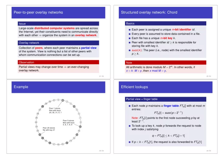
Example
1 2 3 4 5 6 7 8 9 10 11 12 13 14 15 16 17 18 19 20 21 22 23 24 25 26 27 28 29 30 31
Peer9stores fileswithkeys 5,6,7,8,9 Peer1stores fileswithkeys 29,30,31,0,1 Peer20stores filewithkey21
23 / 53
Efficient lookups
Partial view = finger table Each node p maintains a finger table FTp[] with at most m entries: FTp[i] = succ(p +2i1) Note: FTp[i] points to the first node succeeding p by at least 2i1. To look up a key k, node p forwards the request to node with index j satisfying q = FTp[j] k < FTp[j +1] If p < k < FTp[1], the request is also forwarded to FTp[1]
24 / 53