
SLIDE 1
PCA by Projection Pursuit The Package pcaPP
Heinrich Fritz Vienna University of Technology, Austria
Vienna, Austria
June, 2006
Vienna University of Technology
Joint work with . . .
- P. Filzmoser
Department of Statistics and Probability Theory Vienna University of Technology, Austria
- C. Croux
Department of Applied Economics K.U. Leuven, Belgium
M.R. Oliveira
Department of Mathematics Instituto Superior T´ ecnico, Lisbon, Portugal
- K. Kalcher
Vienna University of Technology, Austria
Agenda
- Principal components
- Robust approaches
- The implementation
- Supporting methods
- Covariance estimation by PCAs
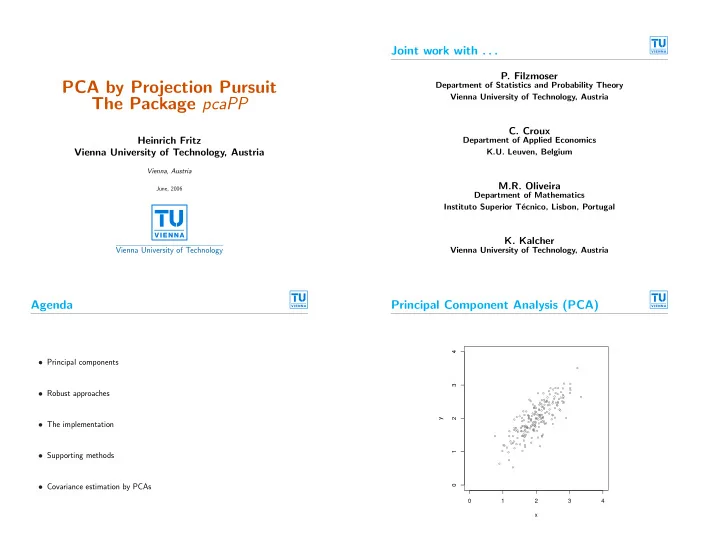
Principal Component Analysis (PCA)
1 2 3 4 1 2 3 4 x y