Path Integral (Auxiliary Field) Monte Carlo approach to ultracold - - PowerPoint PPT Presentation

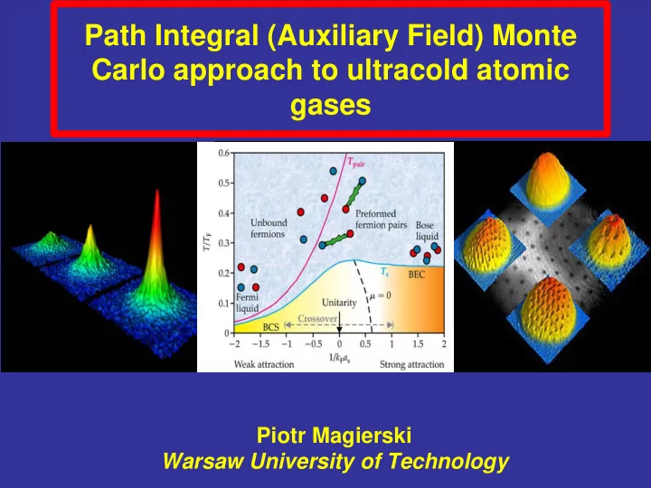
Path Integral (Auxiliary Field) Monte Carlo approach to ultracold atomic gases

Piotr Magierski Warsaw University of Technology

Collaborators:

• A. Bulgac - University of Washington

J.E. Drut - University of North Carolina K.J. Roche – PNNL

• G. Wlazłowski - Univ. of Washington/Warsaw Univ. of Techn.

Outline

• BCS-BEC crossover. Unitary regime.
• Theoretical approach: Path Integral Monte Carlo (QMC)
• Equation of state for the Fermi gas in the unitary
• regime. Critical temperature.
• Correlation functions from QMC: analytic continuation and

inverse problem.

• Pairing gap and pseudogap.
• Viscosity, spin conductivity and diffusion.

A gas of interacting fermions is in the unitary regime if the average separation between particles is large compared to their size (range of interaction), but small compared to their scattering length. n - particle density

n |a|3 >> 1 n r0

3 << 1 r0 - effective range a - scattering length

NONPERTURBATIVE REGIME

System is dilute but strongly interacting! What is a unitary gas? Universality:

   

; x=

FG F

T E x x E   

(0) 0.376(5)  

FG

E

• Energy of noninteracting Fermi gas
• Exp. estimate

One fermionic atom in magnetic field

F

F m

; F I J J L S    

Nuclear spin Electronic spin Collision of two atoms: At low energies (low density of atoms) only L=0 (s-wave) scattering is effective. Two hypefine states are populated in the trap

• Due to the high diluteness atoms in the same hyperfine

state do not interact with one another.

• Atoms in different hyperfine states experience interactions
• nly in s-wave.

2 2 1 1 1 2

( ) ( ) ( ) 2 , ( )

hf Z d i i i hf hf Z e z n z

p H V V V r P V r P V a V I J V J I B   



         



Regal and Jin, PRL 90 90, , 230404 (2003)

Fes eshb hbac ach h res eson

• nance

ance

Tiesinga, Verhaar, Stoof, Phys. Rev. A47 47, 4114 (1993)

Channel coupling

Interatomic distance

E 

resonance: a 

M.W. Zwierlein et al., Nature, 435, 1047 (2005) 6

system of fermionic atoms Li

Feshbach resonance: B=834G BEC side: a>0 BCS side: a<0 UNITARY REGIME

4

• contact

lim ( ) ,

k

C

C n k k





Shina Tan, Ann.Phys.323,2971(2008), Ann.Phys.323,2952(2008)

 

3 2 2 3 4 1 2

( ) 2 2 (1/ ) 4

s S

d k k C E n k m k dE C d a m

 

 



               

 

Total energy

• f the system

Adiabatic relation

C and 1/a are conjugate thermodynamic variables 1/a – „generalized force” C - „generalize displacement” – capture physics at short length scales.

Other theory papers: Tan, Leggett, Braaten, Combescot, Baym, Blume, Werner, Castin, Randeria,Strinati,…

3 ENERGY: ( ) ( ) ; 5

F F

T E x x N x     

2 PRESSURE: ( ) 5 2 3

F

E N P x V V PV E        

Note the similarity to the ideal Fermi gas

Path Integral Monte Carlo for fermions on 3D lattice

• Spin up fermion:
• Spin down fermion:

External conditions:

• temperature
• chemical potential

T 

;

cut

k x x    

L –limit for the spatial correlations in the system

Coordinate space

3

Volume L lattice spacing x   

Periodic boundary conditions imposed

 

2 3 † 3 3 †

ˆ ˆ ˆ ˆ ˆ ˆ ˆ ( ) ( ) ( ) ( ) 2 ˆ ˆ ˆ ˆ ˆ ˆ ( ) ( ) ; ( ) ( ) ( )

s s s s s s

H T V d r r r g d r n r n r m N d r n r n r n r r r    

    

              

   

Hamiltonian

Path Integral Monte Carlo for Fermions on 3D lattice Momentum space

            

UV IR 2 2 2 2

UV momentum cutoff 2 IR momentum cutoff , 2 2

IR UV F

x L m m

ky kx 2π/L

x   x  

k

kcut=π/Dx

2π/L

n(k)

REAL SPACE MOMENTUM SPACE FFT

 

2 3 † 3 3 †

ˆ ˆ ˆ ˆ ˆ ˆ ˆ ( ) ( ) ( ) ( ) 2 ˆ ˆ ˆ ˆ ˆ ˆ ( ) ( ) ; ( ) ( ) ( )

s s s s s s

H T V d r r r g d r n r n r m N d r n r n r n r r r    

    

              

   

2 2 2

1 4 2

cut

mk m g a     

Running coupling constant g defined by lattice

Hamiltonian

2

1

• UNITARY LIMIT

2 m g x   

     

3 ( ) 1 1

ˆ ˆ ˆ ˆ ˆ ˆ ˆ exp exp / 2 exp( )exp / 2 ( ) 1 ˆ ˆ ˆ exp( ) 1 ( ) ( ) 1 ( ) ( ) , exp( ) 1 2 ˆ ˆ ( ) ( ); ˆ (

r r N j j j

H N T N V T N O V r An r r An r A g U W W





              

   

                                   

  

   

ˆ ˆ ˆ ˆ ˆ ˆ ) exp / 2 1 ( ) ( ) 1 ( ) ( ) exp / 2

r

T N r An r r An r T N      

 

                      



Discrete Hubbard-Stratonovich transformation σ-fields fluctuate both in space and imaginary time



     

                

   

             

      

{ ( ,1) 1} { ( ,2) 1} { ( , ) 1} 2

ˆ ( ) ( , ) Tr ({ }); 1 ( , ) ... ; ˆ ˆ ({ }) exp{ [ ({ }) ]} ˆ ˆ Tr ({ }) ˆ ( , )Tr ({ }) ( ) ˆ ( ) Tr ({ }) ˆ ˆ Tr ({ }) {det[1 ( )]}

r r r N

Z T D r U D r N T U T d h HU D r U E T Z T U U U      

  

            



* 3 ,

exp[ ({ })] ({ }) exp( ) ( , ) ( , ) ( ) ( ), ( ) 1 ({ })

c

k l k k l k k l

S U ik x n x y n x y x y x U L

No sign problem!

All traces can be expressed through these single-particle density matrices

One-body evolution

• perator in imaginary time

1kT

 

              



ˆ ˆ ˆ ({ }) exp{ [ ({ }) ]}; ({ })

• ne-body operator

ˆ ({ }) ({ }) ;

• single-particle wave function

kl k l l

U T d h h U U



   



  

[ ]

energy associated with a given sigma field

[ ( , )] ˆ ( ) [ ({ })] ( ) [ ({ })]-

S

D r e E T H E U Z T E U

Sigma space sampling

 

[ ]

( )

S

P e









Quantum Monte-Carlo:

 

1

1 ( ) ({ })

N k k

E T E U N













2 2

( ) - stochastic variable ( ) ( ) 1 ( ) ( )

• number of

uncorrelated samples E T E T E T E T E T N N

 

  

Details of calculations, improvements and problems

• Currently we can reach 143 lattice and perform calcs. down to x = 0.06

(x – temperature in Fermi energy units) at the densities of the order of 0.03.

• Effective use of FFT(W) makes all imaginary time propagators diagonal (either in

real space or momentum space) and there is no need to store large matrices.

• Update field configurations using the Metropolis importance sampling algorithm.

QMC calculations can be split into two independent processes: 1) sample generation (generation of sigma fields), 2) calculations of observables.

• Change randomly at a fraction of all space and time sites the signs the auxiliary

fields σ(r,) so as to maintain a running average of the acceptance rate between 0.4 and 0.6 .

• At low temperatures use Singular Value Decomposition of the evolution operator

U({σ}) to stabilize the numerics.

• MC correlation “time” ≈ 200 time steps at T ≈ Tc for lattices 103 .

Unfortunately when increasing the lattice size the correlation time also increases.

One needs few thousands uncorrelated samples (we usually take about 10 000) to

decrease the statistical error to the level of 1%.

Finite size scaling: Effective range corrections: CM corrections:

0.4 0.5

F eff

k r  

0.671 0.8    

Bulgac, Drut, Magierski, PRA78, 023625(2008), Wlazłowski, Magierski, Bulgac, Drut, Roche, arXive:1212.1503 (to appear in Phys. Rev. Lett.)

Total systematic error does not exceed 10-15%

CM momentum

• f a fermion pair

• S. Nascimbene et al.

Nature 463, 1057 (2010)

Courtesy of C. Salomon

QMC

Bulgac, Drut, Magierski, PRL99, 120401(2006)

Experiment

• Diagram. MC

Burovski et al. PRL96, 160402(2006)

• Diagram. + analytic

Haussmann et al. PRA75, 023610(2007)

exp( )  

Experiment: M.J.H. Ku, A.T. Sommer, L.W. Cheuk, M.W. Zwierlein , Science 335, 563 (2012) QMC (PIMC + Hybrid Monte Carlo): J.E.Drut, T.Lähde, G.Wlazłowski, P.Magierski, Phys. Rev. A 85, 051601 (2012)

Equation of state of the unitary Fermi gas - current status

Local density approximation (LDA) from QMC

3 ( ) 5

F

F N x N N         

Uniform system

3 2 2/3 2

3 ( ) ( ( )) ( ) ( ) 5 ( ) ; ( ) 3 ( ) ( ) 2

F F F

d r r x r U r n r T x r r n r r m                      



Nonuniform system (gradient corrections neglected)

( ) ( ( )) ( ) ( ) ( ) F N x r U r n r n r              

The overall chemical potential and the temperature T are constant throughout the system. The density profile will depend on the shape of the trap as dictated by:



Using as an input the Monte Carlo results for the uniform system and experimental data (trapping potential, number of particles), we determine the density profiles.

Entropy as a function of energy (relative to the ground state) for the unitary Fermi gas in the harmonic trap.

Comparison with experiment

John Thomas’ group at Duke University,

L.Luo, et al. Phys. Rev. Lett. 98, 080402, (2007)

THEORY Theory: EXP.

Ratio of the mean square cloud size at B=1200G to its value at unitarity (B=840G) as a function of the energy. Experimental data are denoted by point with error bars.

THEORY

ho F

E N  1200 1/ 0.75

F

B G k a    

Static and dynamic responses from QMC

   

( ) ( ) '/ '/

ˆ ˆ ˆ ( ) ( ) ( ) ( ') ( ') ˆ ˆ ( ) ( ) [ ( ), ] ' ( ') ' ( ') ( ) 1 1 2 ' 2 '

T T

H t H AX t B t i dt t t X t t i t A t B d A d A e e i i

 

            

          

               

  

1/

ˆ ˆ ˆ ( ) ˆ ˆ ˆ ˆ ˆ ( ) ;

T

H t H AX B X d A B A A A              



Static: Dynamic:

Constraints :

Examples od useful spectral function::

Shear viscosity Spin conductivity

Linear inverse problem G is known from QMC with some error for a number of values of y, usually uniformly distributed within the interval: (0, 1/T) Constraints:

SVD method: Effects of noise:

Magierski, Wlazłowski, Comp. Phys. Comm. 183 (2012) 2264

Maximum entropy method (MEM): Bayes’ theorem: Maximization of conditional probability: Relative entropy term

Magierski, Wlazłowski, Comp. Phys. Comm. 183 (2012) 2264

Magierski, Wlazłowski,

• Comp. Phys. Comm. 183 (2012) 2264

Spectral weight function at unitarity:

1

( )

F

k a

 

0.12

F

T   0.15

F C

T T    0.17

F

T   0.21 F T  

Results in the vicinity

• f the unitary limit:
• Critical temperature
• Ground state energy
• Pairing gap

Bulgac, Drut, Magierski, PRA78, 023625(2008)

From Sa de Melo, Physics Today (2008)

Pairing pseudogap: suppression of low-energy spectral weight function due to incoherent pairing in the normal state (T >Tc)

Important issue related to pairing pseudogap:

• Are there sharp gapless quasiparticles in a normal Fermi liquid

YES: Landau’s Fermi liquid theory; NO: breakdown of Fermi liquid paradigm

Magierski, Wlazłowski, Bulgac, Phys. Rev. Lett.107,145304(2011) Magierski, Wlazłowski, Bulgac, Drut, Phys. Rev. Lett.103,210403(2009)

Gap in the single particle fermionic spectrum - theory

RF spectroscopy in ultracold atomic gases

Stewart, Gaebler, Jin, Using

photoemission spectroscopy to probe a strongly interacting Fermi gas, Nature, 454, 744 (2008)

Experiment (blue dots): D. Jin’s group Gaebler et al. Nature Physics 6, 569(2010) Theory (red line): Magierski, Wlazłowski, Bulgac, Phys.Rev.Lett.107,145304(2011)

Hydrodynamics at unitarity

Scaling:

 

1 2 2 1 2 3 /2

1 , ,..., , ,..., ;

N i i N i i N

r E r r r r r E               

Consequence: uniform expansion does not produce entropy = bulk viscosity is zero!

Shear viscosity:

4

B

S k   

KSS conjecture

Kovtun,Son,Starinets, Phys.Rev.Lett. 94, 111601, (2005) from AdS/CFT correspondence

For any physical fluid: Perfect fluid - strongly interacting quantum system =

4

B

S k   

Maxwell classical estimate: ~ mean free path



Candidates: unitary Fermi gas, quark-gluon plasma

No well defined quasiparticles

x

v F A y    

x y

No intrinsic length scale Uniform expansion keeps the unitary gas in equilibrium

Additional symmetries and sum rules: 𝜁 − energy density Combined Maximum Entropy and SVD methods were applied

G.Wlazłowski, P.Magierski,J.E.Drut,

• Phys. Rev. Lett. 109, 020406 (2012)

Uncertainties related to numerical analytic continuation

Shear viscosity to entropy ratio – experiment vs. theory

(from A. Adams et al.1205.5180)

QMC calculations for UFG:

• G. Wlazłowski, P. Magierski, J.E. Drut,
• Phys. Rev. Lett. 109, 020406 (2012)

Lattice QCD ( SU(3) gluodynamics ): H.B. Meyer, Phys. Rev. D 76, 101701 (2007)

Spin susceptibility, spin conductivity, spin diffusion

Wlazłowski, Magierski, Bulgac, Drut, Roche, arXive:1212.1503, to appear in Phys. Rev. Lett. (2013)

Wlazłowski, Magierski, Bulgac, Drut, Roche, arXive:1212.1503, to appear in Phys. Rev. Lett. (2013)

Cold atomic gases and high Tc superconductors

From Fischer et al., Rev. Mod. Phys. 79, 353 (2007) & P. Magierski, G. Wlazłowski, A. Bulgac, Phys. Rev. Lett. 107, 145304 (2011)

0.5 0.16

F c F

T     