Particle-Based Fluid Simulation CSE169: Computer Animation Steve - PowerPoint PPT Presentation
Particle-Based Fluid Simulation CSE169: Computer Animation Steve Rotenberg UCSD, Winter 2019 Del Operations Del: = Gradient: =
Particle-Based Fluid Simulation CSE169: Computer Animation Steve Rotenberg UCSD, Winter 2019
Del Operations 𝜖 𝜖 𝜖 • Del: 𝛼 = 𝜖𝑦 𝜖𝑧 𝜖𝑨 𝜖𝑡 𝜖𝑡 𝜖𝑡 • Gradient: 𝛼𝑡 = 𝜖𝑦 𝜖𝑧 𝜖𝑨 𝜖𝑤 𝑧 = 𝜖𝑤 𝑦 𝜖𝑧 + 𝜖𝑤 𝑨 • Divergence: 𝛼 ∙ 𝐰 𝜖𝑦 + 𝜖𝑨 𝜖𝑤 𝑧 𝜖𝑤 𝑧 𝜖𝑤 𝑨 𝜖𝑤 𝑦 𝜖𝑨 − 𝜖𝑤 𝑨 𝜖𝑦 − 𝜖𝑤 𝑦 • 𝜖𝑧 − Curl: 𝛼 × 𝐰 = 𝜖𝑨 𝜖𝑦 𝜖𝑧 = 𝜖 2 𝑡 𝜖𝑦 2 + 𝜖 2 𝑡 𝜖𝑧 2 + 𝜖 2 𝑡 𝛼 2 𝑡 • Laplacian: 𝜖𝑨 2
Transport Equations 𝑒𝑡 • Advection: 𝑒𝑢 = −𝐰 ∙ 𝛼𝑡 𝑒𝐰 • Convection: 𝑒𝑢 = −𝐰 ∙ 𝛼𝐰 𝑒𝑡 𝑒𝑢 = 𝑙𝛼 2 𝑡 • Diffusion: 𝑒𝐰 𝑒𝑢 = 𝜈𝛼 2 𝐰 • Viscosity: 𝑒𝐰 • Pressure: 𝑒𝑢 = −𝛼𝑞
Navier-Stokes Equation • The incompressible Navier-Stokes equation describes the forces on a fluid as the sum of convection, viscosity, and pressure terms: 𝜖𝐰 𝜖𝑢 = −𝐰 ∙ 𝛼𝐰 + 𝜈𝛼 2 𝐰 −𝛼𝑞 • In addition, we also have the incompressibility constraint: 𝛼 ∙ 𝐰 = 0 • As discussed in the previous lecture, these are formulated from the point of view of a fixed point in space (Eulerian frame of reference)
Lagrangian Approach • In the Lagrangian approach, we formulate the Navier-Stokes equation from the point of view of a particle moving along with the fluid • The pressure and viscosity terms don’t change, but the convection term goes away entirely 𝑒𝐰 𝑒𝑢 = 𝜈𝛼 2 𝐰 −𝛼𝑞 • 1 𝜍 The paper also adds a term for externally applied forces as well as a Τ term to account for the fact that the particle based methods will have some variation in density 𝑒𝐰 𝑗 𝑒𝑢 = 𝜈𝛼 2 𝐰 𝑗 − 1 𝛼𝑞 𝑗 + 𝐠 𝑗 𝜍 𝑗 𝑛 𝑗
Particle-Based Fluids
Grid-Based Methods • Fluid dynamics has traditionally been simulated on uniform grids or irregular meshes • These techniques are good for engineering applications due to their potential for high accuracy • They are effective in computer graphics uses as well, particularly for smoke and simulations of airflows • However, it is very difficult to handle fluid interfaces (such as the water-air boundary) and complex splashing situations, which are the situations one often wants in entertainment applications
Smooth Particle Hydrodynamics • Particle based fluid simulation is often referred to as smooth particle hydrodynamics or SPH • Some of the original work was done for simulating galactic gas dynamics by astrophysicists • The technique was introduced to the computer graphics community around 2003 • In recent years, advances in the techniques as well as increases in GPU computational power have made large-scale SPH simulations possible • The technique has proven very effective, especially for simulating very dynamic situations with lots of splashing and interaction with complex surfaces
SPH Fluids in Computer Graphics • We will follow the paper “SPH Fluids in Computer Graphics” • Authors: Markus Ihmsen, Jens Orthmann, Barbara Solenthaler, Andreas Kolb, Matthias Teschner • This was a ‘State of The Art Report’ (STAR) published in Eurographics 2014, and it summarizes much of the development on the subject that had been done in the previous 10 years • This is a great overview of the subject and the important issues, and with lots of other great references in the bibliography • Many of the formulas in these slides come from the paper as well as a few quoted statements
Field Representation • We saw that scalar and vector fields can be represented by grids or meshes by sampling the field at the grid points and interpolating the values in between • Alternately can use a meshless set of irregularly spaced particles to represent a field • Rather than being a 0 dimensional point, a particle is thought of as being smeared out over some small radius • The maximum radius of influence for a particle is called the support radius • The particles have to be close enough together so that they effectively cover all of the domain of interest, and often they are arranged so that every point in the domain is overlapped by several particles (maybe around 3-10)
Field Representation • Each particle 𝑗 represents a small sample of the fluid so it will have a mass 𝑛 𝑗 , position 𝐲 𝑗 , and velocity 𝐰 𝑗 • We will also compute various properties per particle such as the local density 𝜍 𝑗 , pressure 𝑞 𝑗 , or volume 𝑊 𝑗
Kernel Function • We define a kernel function W () that represents the strength of a particle’s influence as a function of the distance from the particle • At the support radius, we expect W () to go to 0 and smoothly increase to 1 as we get closer to the particle • There have been many kernel functions proposed, and we will look at the one used in the paper
Kernel Function • “A quantity 𝐵 𝑗 at arbitrary position 𝐲 𝑗 is approximately computed with a set of known quantities 𝐵 𝑘 at neighboring particle positions 𝐲 𝑘 ” 𝑛 𝑘 𝐵 𝑗 = 𝐵 𝑘 𝑋 𝑗𝑘 𝜍 𝑘 𝑘 • With 𝑋 𝑗𝑘 being a kernel function of the form 𝐲 𝑗 − 𝐲 𝑘 = 𝑋 𝑟 = 1 𝑋 𝑗𝑘 = 𝑋 ℎ 𝑒 𝑔 𝑟 ℎ • A typical choice for the function f () would be 2 3 − 𝑟 2 + 1 2 𝑟 3 0 ≤ 𝑟 < 1 3 1 ≤ 2 𝑔 𝑟 = 1 6 2 − 𝑟 3 2𝜌 𝑟 ≥ 2 0
Kernel Function 𝐲 𝑗 − 𝐲 𝑘 = 𝑋 𝑟 = 1 𝑋 𝑗𝑘 = 𝑋 ℎ 𝑒 𝑔 𝑟 ℎ • The value d is the number of dimensions • The value h is the smoothing radius , which is not the same as the support radius • The particle spacing is typically close to h • From examining the equations, one can see that the support radius is 2 h in the example from the paper, but they mention it may vary from h to 3 h depending on choice of kernel function f ()
Derivative Computation • When using uniform grids, we were able to easily compute various spatial derivatives by using finite differencing • With particles, the irregular spacing makes derivative computation a little more tricky and several approaches have been used in the literature • The paper uses the following: 2 + 𝐵 𝑘 𝐵 𝑗 𝛼𝐵 𝑗 = 𝜍 𝑗 𝑛 𝑘 𝛼𝑋 𝑗𝑘 2 𝜍 𝑗 𝜍 𝑘 𝑘 𝛼 ∙ 𝐁 𝑗 = − 1 𝑛 𝑘 𝐁 𝑗𝑘 ∙ 𝛼𝑋 𝑗𝑘 𝜍 𝑗 𝑘 𝑛 𝑘 𝐲 𝑗𝑘 ∙ 𝛼𝑋 𝑗𝑘 𝛼 2 𝐵 𝑗 = 2 𝐵 𝑗𝑘 𝐲 𝑗𝑘 ∙ 𝐲 𝑗𝑘 + 0.01ℎ 2 𝜍 𝑘 𝑘
Derivative Computation • Notice that all of the derivatives involve summing over j , which is the set of nearby particles within the support radius • In order to do the calculations, every particle must determine which particles are nearby • This can be problematic when you are dealing with millions of particles, and so special data structures are required to make this neighbor search fast • We will look at those in a little bit
Equations of Motion • SPH uses the Lagrangian form of the Navier-Stokes equation: 𝑒𝐰 𝑗 𝑒𝑢 = 𝜈𝛼 2 𝐰 𝑗 − 1 𝛼𝑞 𝑗 + 𝐠 𝑗 𝜍 𝑗 𝑛 𝑗 • This is computed for each particle and then integrated using the standard forward Euler method of integration that we’ve been using for other particle systems • Note that it requires a density 𝜍 and pressure p to be calculated first and the paper has a couple different methods to do that depending on the specific approach
Algorithm • The paper presents 4 different algorithms for SPH simulation • They are all similar and effectively try to calculate the same thing, but they use different computational approaches and don’t produce the exact same results • The main difference between the approaches involves the exact order that things are done and how the incompressibility constraint is handled • Most methods allow for some compression, but some of the better approaches attempt to enforce incompressibility using iterative approaches or solutions to large systems of equations • In general, the more sophisticated methods require more time to compute a single time step, but run more stable and can handle larger time steps • The result is that usually the more sophisticated approaches will outperform the simpler approaches in real world use cases
Integration & Time Steps • We need small time steps to keep things stable, but ideally we could use larger time steps if things aren’t moving as quickly • We can therefore consider adapting the time step over time based on what is happening in the simulation • It is common to base this off of the Courant-Friedrich- Levy (CFL) condition that limits the time step so that the fastest particle doesn’t move more than some portion of it’s smoothing radius: ℎ ∆𝑢 ≤ 𝜇 with 𝜇 ≈ 0.4 𝐰 𝑛𝑏𝑦
Spatial Hash Tables
Recommend
More recommend
Explore More Topics
Stay informed with curated content and fresh updates.
