Partial Model Construction Given a clause set N and an ordering we - PowerPoint PPT Presentation

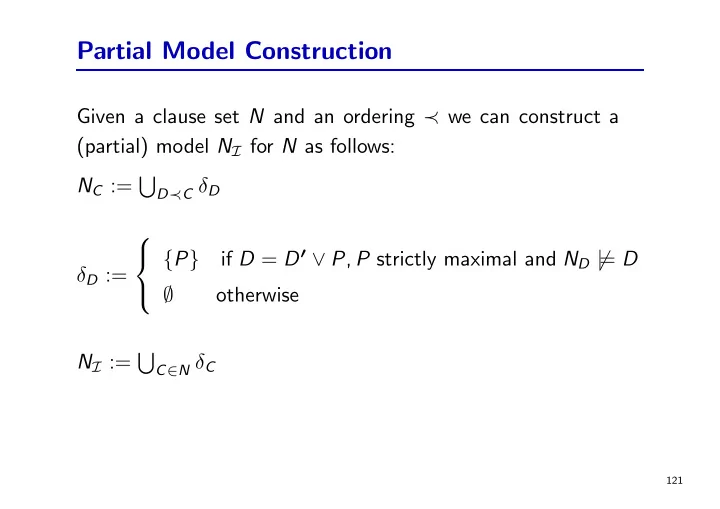
Partial Model Construction Given a clause set N and an ordering ≺ we can construct a (partial) model N I for N as follows: N C := � D ≺ C δ D  if D = D ′ ∨ P , P strictly maximal and N D �| { P } = D  δ D := ∅ otherwise  N I := � C ∈ N δ C 121

Partial Model Construction Clauses C with δ C � = ∅ are called productive. Some properties of the partial model construction. Proposition 2.12: 1. For every D with ( C ∨ ¬ P ) ≺ D we have δ D � = { P } . 2. If δ C = { P } then N C ∪ δ C | = C . = D then for all C ′ with C ≺ C ′ we have N C ′ | 3. If N C | = D and in particular N I | = D . 122

Notation: N , N ≺ C , N I , N C Please properly distinguish: • N is a set of clauses intepreted as the conjunction of all clauses. • N ≺ C is of set of clauses from N strictly smaller than C with respect to ≺ . • N I , N C are sets of atoms, often called Herbrand Interpreta- tions. N I is the overall (partial) model for N , whereas N C is generated from all clauses from N strictly smaller than C . • Validity is defined by N I | = P if P ∈ N I and N I | = ¬ P if P �∈ N I , accordingly for N C . 123

Superposition The superposition calculus consists of the inference rules superposition left and factoring: Superposition Left ( N ⊎ { C 1 ∨ P , C 2 ∨ ¬ P } ) ⇒ ( N ∪ { C 1 ∨ P , C 2 ∨ ¬ P } ∪ { C 1 ∨ C 2 } ) where P is strictly maximal in C 1 ∨ P and ¬ P is maximal in C 2 ∨ ¬ P Factoring ( N ⊎ { C ∨ P ∨ P } ) ⇒ ( N ∪ { C ∨ P ∨ P } ∪ { C ∨ P } ) where P is maximal in C ∨ P ∨ P 124

Superposition examples for specific redundancy rules are Subsumption ( N ⊎ { C 1 , C 2 } ) ⇒ ( N ∪ { C 1 } ) provided C 1 ⊂ C 2 Tautology Deletion ( N ⊎ { C ∨ P ∨ ¬ P } ) ⇒ ( N ) Subsumption Resolution ( N ⊎ { C 1 ∨ L , C 2 ∨ ¯ L } ) ⇒ ( N ∪ { C 1 ∨ L , C 2 } ) where C 1 ⊆ C 2 125

Superposition Theorem 2.13: If from a clause set N all possible superposition inferences are redundant and ⊥ / ∈ N then N is satisfiable and N I | = N . 126

Superposition So the proof actually tells us that at any point in time we need only to consider either a superposition left inference between a minimal false clause and a productive clause or a factoring inference on a minimal false clause. 127

A Superposition Theorem Prover STP 3 clause sets: N(ew) containing new inferred clauses U(sable) containing reduced new inferred clauses clauses get into W(orked) O(ff) once their inferences have been computed Strategy: Inferences will only be computed when there are no possibilities for simplification 128

Rewrite Rules for STP Tautology Deletion ( N ⊎ { C } ; U ; WO ) ⇒ STP ( N ; U ; WO ) if C is a tautology Forward Subsumption ( N ⊎ { C } ; U ; WO ) ⇒ STP ( N ; U ; WO ) if some D ∈ ( U ∪ WO ) subsumes C Backward Subsumption U ( N ⊎ { C } ; U ⊎ { D } ; WO ) ⇒ STP ( N ∪ { C } ; U ; WO ) if C strictly subsumes D ( C ⊂ D ) 129

Rewrite Rules for STP Backward Subsumption WO ( N ⊎ { C } ; U ; WO ⊎ { D } ) ⇒ STP ( N ∪ { C } ; U ; WO ) if C strictly subsumes D ( C ⊂ D ) Forward Subsumption Resolution ( N ⊎ { C 1 ∨ L } ; U ; WO ) ⇒ STP ( N ∪ { C 1 } ; U ; WO ) if there exists C 2 ∨ ¯ L ∈ ( UP ∪ WO ) such that C 2 ⊆ C 1 Backward Subsumption Resolution U ( N ⊎ { C 1 ∨ L } ; U ⊎ { C 2 ∨ ¯ L } ; WO ) ⇒ STP ( N ∪ { C 1 ∨ L } ; U ⊎ { C 2 } ; WO ) if C 1 ⊆ C 2 130

Rewrite Rules for STP Backward Subsumption Resolution WO ( N ⊎ { C 1 ∨ L } ; U ; WO ⊎ { C 2 ∨ ¯ L } ) ⇒ STP ( N ∪ { C 1 ∨ L } ; U ; WO ⊎ { C 2 } ) if C 1 ⊆ C 2 Clause Processing ( N ⊎ { C } ; U ; WO ) ⇒ STP ( N ; U ∪ { C } ; WO ) Inference Computation ( ∅ ; U ⊎ { C } ; WO ) ⇒ STP ( N ; U ; WO ∪ { C } ) where N is the set of clauses derived by superposition inferences from C and clauses in WO . 131

Soundness and Completeness Theorem 2.14: ( N ′ ∪ {⊥} ; U ; WO ) ⇒ ∗ N | = ⊥ ⇔ ( N ; ∅ ; ∅ ) STP Proof in L. Bachmair, H. Ganzinger: Resolution Theorem Proving appeared in the Handbook of Automated Reasoning, 2001 132

Termination Theorem 2.15: For finite N and a strategy where the reduction rules Tautology Deletion, the two Subsumption and two Subsumption Resolution rules are always exhaustively applied before Clause Processing and Inference Computation, the rewrite relation ⇒ STP is terminating on ( N ; ∅ ; ∅ ). Proof: think of it (more later on). 133

Fairness Problem: STP ( N ′ ∪ {⊥} ; U ; WO ) . If N is inconsistent, then ( N ; ∅ ; ∅ ) ⇒ ∗ Does this imply that every derivation starting from an inconsistent set N eventually produces ⊥ ? No: a clause could be kept in U without ever being used for an inference. 134

Fairness We need in addition a fairness condition: If an inference is possible forever (that is, none of its premises is ever deleted), then it must be computed eventually. One possible way to guarantee fairness: Implement U as a queue (there are other techniques to guarantee fairness). With this additional requirement, we get a stronger result: If N is inconsistent, then every fair derivation will eventually produce ⊥ . 135