Part I If you want to save or load a file, you need to know what the - - PowerPoint PPT Presentation

Data Analysis and Visualization with R

André Batista, Ph.D. Student andrefmb@usp.br 2016

Source: http://cns.iu.edu/images/teaching/ivmoocbook14/IVMOOC_Book_Preview.html

R Programming Language Fundamentals

Variables & Data Structures

Data Visualization with ggplot2 Data Analysis

Statistical Testing and Prediction Exploratory Analysis AGENDA

This content , available at http://varianceexplained.org/RData/code/code_lesson1/ Others references are cited in the proper slides

Part I

R Fundamentals

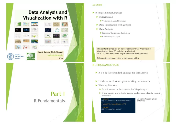
R - FUNDAMENTALS R is a de facto standard language for data analysis Firstly, we need to set up our working environment Working directory

Default location on the computer that R is pointing at If you want to save or load a file, you need to know what the current directory is

We use the functions getwd() and setwd()

R - VARIABLES Variables

Most basic and crucial element of R Single numbers, vectors, matrix, data frame are the most used variables

Examples

Primitively, R can be used as a scientific calculator

R - VECTORS We can create a vector consisting of multiple numeric values by using a function c( ) Subset the vector and using APPEND( ) function

* after = <<position>>

R - VECTORS A lot of statistical programming in R relies on mathematical

• perations applied to a vector a matrix

Basic calculator-like functions may apply to all elements in a given vector Operations between two vectors

Inner product Vectors must have the same length

R - VECTORS We can use the function CLASS( ) to check the class of an element We can populate a vector using SEQ( ) function

random generation for the normal distribution

R - VECTORS We can use relational and logical operator for selecting elements in a vector REP( ) function R - VECTORS Summary Statistics of Vectors

Generated boxplot for x

R - VECTORS Names

Elements in a vector have names! And we can access them using the function NAMES( ) NULL implies that the elements in the vector currently do not have Now we have

R - MATRICES Matrices are like two-dimensional vectors, organizing values into rows and columns The easiest way to create a matrix is using MATRIX( ) A matrix cannot contain multiple data types Here, both MA and MB contain only numeric values

R - MATRICES Combining

Sometimes we want to combine different matrices and vectors We can use CBIND( ) and RBIND( ) functions

As long as their lengths and dimensions are comparable. Example of error: Combining MA and MB into a new matrix M

R - MATRICES Extracting values from matrices is straightforward Obtaining info about a matrix Setting ROWNAME and COLNAME R - ARRAYS An array in R can have one, two or more dimensions It is simply a vector which is stored with additional atributes giving the dimensions and optionally names for those dimensions

dim=c(3,4,2) means TWO dimensions having a matrix with FOUR columns and THREE rows each Now, try this:

ar1 <- array(1:24, dim=c(3,4,2)) ar1[,2:3,] ar1[2,,1] sum(ar1[,,1]) sum(ar1[1:2,,1])

R LISTS and DATA FRAMES Lists and Data frames

Matrices are extremely useful for processing and storing large datasets

But have several limitations that may not suit our needs (one datatype

• nly, for example)

List

It is a vector containing other

• bjects which may be of different

data types or different lengths

R LISTS and DATA FRAMES Data Frames

Data frames are lists with a set of restrictions It is a list of vectors which are conveniently arranged as columns All vectors or columns in a data frame must have the same length Data frames mimic matrices when needed and appropriate

MTCARS

R comes with built-in datasets. MTCARS contains statistics about 32 cars in 1974 Use the command View(mtcars) to display the data in a spreadsheet

R LISTS and DATA FRAMES

If you want to see only the first 6 rows, you can use the head( ) function One of the first steps when we have a data frame or a dataset is try to understand about its statistics

DATA FRAMES We can retrieve a specific column by name, using $columnname

Or you can use mtcars

• r still mtcars[, 1]

We can also obtain multiple rows at once as well: mtcars[1:3, ]

How to create a new data frame?

Using data.frame function

MISSING VALUES In R missing values are represented by the symbol (NA not available)

Impossible values (e.g., dividing by zero) are represented by NaN

We have functions to deal with NA values, as follows:

GUIDED EXERCISE Here we will learn by practicing with an example We will learn

How to load files into R (e.g., CSV files) How to deal with NA values How to apply functions into a data frame How to plot basic graphics

Firstly, you need to download the grades.csv from Save the file into R workspace

This exercise is based on http://www.utsc.utoronto.ca/~sdamouras/summer/Rworkshop1.pdf

Exercise Part I Firstly, we need to load Grades.csv into a new data frame We have NA values in our data frame. For example, Quiz.9 is a NA

• column. We can create a new grade data frame without column 13

(quiz 9) grade[ , -13] Exercise Part II The next step is another approach for dealing with NA values. Here we will replace all NA values for zero How we can get the sum of all quizzes for each student?

We can use the APPLY( ) function

Exercise Part III So, if we want to apply a sum, we will use FUN = sum and this function must be applied to all rows, so MARGIN = 1

quiz.sum = apply(X=grade2[, 5:12], MARGIN = 1, FUN = sum)

Now we have the sum of all quizzes for each student!

Exercise Part IV Now, we can calculate the final grade Final.grade What about to discover how good were the student final grade? We can generate a histogram for this!

Final.grade = quiz.sum/80*20 + grade2$Midterm.1/50*15 + grade2$Midterm.2/50*15 + grade$Final.Exam/100*50 Final.grade <- round(Final.grade, 0)

Exercise Part V Histogram

hist(Final.grade)

Exercise Part VI BoxPlot

boxplot(Final.grade)

Exercise Part VII We can now assign concepts for our students! For example:

FinalGrade < 50 50 <= FinalGrade < 60 60 <= FinalGrade < 70 70 <= FinalGrade < 80 FinalGrade >= 80

Exercises - VIII Now we will generate a barplot Exercise - IX calculate the Midterm for each student and see the relationship between Midterm and Final.Grade

Midterm = (grade2$Midterm.1 + grade2$Midterm.2) /2 plot(Midterm, Final.grade, pch=20)

Exercise - X Lately we will export final grades to a new CSV using write.csv function

write.csv(Final.grade, file="finalgrade.csv")

Demonstração Adicional

http://andrefmb.sdf.org/cursoR/graficosBasicos.html

Part II

GGPLOT2

Ggplot2 and R

A Picture really is worth a thousand words Visual Analysis let us understand the basic nature

• f the data

We will use ggplot2 a powerful R package that produces data visualizations easily and intuitively ggplot2 is a third package

We have to install it

Each time we reopen R, we need to load this library using

Diamonds

ggplot2 comes with some data available to use as demonstration We will use the Diamonds dataset

It contains information about several attributes of 54000 diamonds We can access it with diamonds Try ?diamonds

View(diamonds)

> ?diamonds

http://www.bluediamondtexas.com/images/diamond-chart.jpg

Scatterplots and Bar Graph

Interesting Questions - Diamonds How does weight, in carats, affect the price? affect the price? How can we determine the relationship between attributes?? We can use, for example, a scatter plot Scatter plot is a type of mathematical diagram using Cartesian coordinates to display values for typically two variables for a set of data [Wikipedia]

Aesthetics

A dimension of a graph that we can perceive visually

Color, size, shape of the points, etc.

Our first visualization

Aesthetics attributes let us communicate some dimension of the data and understand complex relationship between them For our first example, we use ggplot2 to create a scatterplot where we put carat (weight) on the X axis and price, in dollars, on the Y axis ggplot(diamonds, aes(x=carat, y=price)) + geom_point()

Our first visualization

Aesthetics attributes let us communicate some dimension of the data and understand complex relationship between them For our first example, we use ggplot2 to create a scatterplot where we put carat (weight) on the X axis and price, in dollars, on the Y axis

And we obtain

ggplot(diamonds, aes(x=carat, y=price)) + geom_point()

Scatterplot with ggplot2 There are three parts to a ggplot2 graph

• 1. data we will be graphing

in this case we a plotting the diamonds data frame

• 2. Mapping the aesthetics to attributes we will be ploting

in this case we use aes( ) and set that X axis will be carat and Y axis will be price

• 3. Layer: what type of graph it is

In this case we make a scatter plot: the name for that layer is geom_point

geom ggplot(diamonds, aes(x=carat, y=price)) + geom_point()

Ggplot2 Geom Types

https://www.rstudio.com/wp-content/uploads/2015/03/ggplot2-cheatsheet.pdf

Bar Graph ggplot(diamonds, aes(x=clarity, fill=cut)) + geom_bar() Bar Graph ggplot(diamonds, aes(x=clarity, fill=cut)) + geom_bar()

Our second visualization with ggplot2 There are many attributes of the data we can communicate

ggplot(diamonds, aes(x=carat, y=price, color=clarity)) + geom_point()

Our second visualization with ggplot2 There are many attributes of the data we can communicate

ggplot(diamonds, aes(x=carat, y=price, color=clarity)) + geom_point()

Our second visualization with ggplot2 There are many attributes of the data we can communicate

ggplot(diamonds, aes(x=carat, y=price, color=clarity)) + geom_point()

Now every point is colored according to the quality of the clarity of each diamond You can see that some of the lighter diamonds are more expensive if they have a high clarity rating, and conversely that some of the heavier diamonds aren't as expensive for having a low clarity rating.

Our third visualization with ggplot2 If we would rather see how the quality of the color or cut of the diamond affects the price?

We can change the aesthetic

ggplot(diamonds, aes(x=carat, y=price, color=color)) + geom_point()

Our third visualization with ggplot2 If we would rather see how the quality of the color or cut of the diamond affects the price?

We can change the aesthetic

ggplot(diamonds, aes(x=carat, y=price, color=color)) + geom_point()

Add more aesthetic attribute Now, try this:

ggplot(diamonds, aes(x=carat, y=price, color=clarity, size=cut)) + geom_point()

Add more aesthetic attribute Now, try this:

ggplot(diamonds, aes(x=carat, y=price, color=clarity, size=cut)) + geom_point()

Adding Layers

Scatter plot is only one layer of our graph We can add additional layers besides the scatter plot using the sign Try this:

ggplot(diamonds, aes(x=carat, y=price)) + geom_point() + geom_smooth()

Adding Layers

Scatter plot is only one layer of our graph We can add additional layers besides the scatter plot using the sign Try this:

ggplot(diamonds, aes(x=carat, y=price)) + geom_point() + geom_smooth()

geom_smooth() Gray around the curve confidence interval Suggesting how much uncertainty there is in this smoothing curve Linear Method Similarly, if we would rather show a best fit straight line rather than a curve, we can change the "method" option in the geom_smooth layer. In this case it's method="lm", where "lm" stands for "Linear model".

ggplot(diamonds, aes(x=carat, y=price)) + geom_point() + geom_smooth(method="lm")

Linear Method Similarly, if we would rather show a best fit straight line rather than a curve, we can change the "method" option in the geom_smooth layer. In this case it's method="lm", where "lm" stands for "Linear model".

ggplot(diamonds, aes(x=carat, y=price)) + geom_point() + geom_smooth(method="lm")

Faceting Another way we can communicate information about an attribute is to divide our plot up into multiple plot facet_wrap function We put a tilde (~) and then the attribute we would like to

ggplot(diamonds, aes(x=carat, y=price, color=cut)) + geom_point() + facet_wrap(~ clarity)

Faceting

ggplot(diamonds, aes(x=carat, y=price, color=cut)) + geom_point() + facet_wrap(~ clarity)

Faceting We have divided it into eight subplots, each of which has a different clarity value We can even divide our graph based on two different attributes, such as both color and clarity, using facet_grid For example In this case we have: color ~ clarity It means: color explained by clarity Color will be on X axis (row) Clarity on Y axis (column)

ggplot(diamonds, aes(x=carat, y=price, color=cut)) + geom_point() + facet_grid(color ~ clarity)

Fatecing - Grid

ggplot(diamonds, aes(x=carat, y=price, color=cut)) + geom_point() + facet_grid(color ~ clarity)

Ggplot2: Title and Labels There are many other ways to customize a plot Firstly, we want to set a title or set the x or y axis labels manually We change these options adding to the end of the line of code

ggplot(diamonds, aes(x=carat, y=price)) + geom_point() + ggtitle("My scatter plot")

Ggplot2: Title and Labels

ggplot(diamonds, aes(x=carat, y=price)) + geom_point() + ggtitle("My scatter plot") + xlab("Weight (carats)") + ylab("Price (Dollars)")

Limiting ranges We can also limit the range of the x or the y axes

ggplot(diamonds, aes(x=carat, y=price)) + geom_point() + ggtitle("My scatter plot") + xlab("Weight (carats)") + xlim(0, 2) Warning message: Removed 1889 rows containing missing values (geom_point).

Limiting ranges Similarly, if we wanted to show only the y-axis from 0 to 10000

ggplot(diamonds, aes(x=carat, y=price)) + geom_point() + ggtitle("My scatter plot") + xlab("Weight (carats)") + ylim(0,10000) + xlim(0,2)

Histograms and Density Curves

Histograms

Scatter plots are just one kind of graph! Sometimes we want to look at just one dimension

• f our data and observe its distribution: for that,

It is very easy: all you need to do to make a histogram is to change your layer from geom_point( ) to geom_histogram( )

Histograms

ggplot(diamonds, aes(x=price)) + geom_histogram()

Another example

ggplot(diamonds, aes(x=price, fill=clarity)) + geom_histogram()

Histograms: Aesthetic We can change the width of each bin as an options to geom_histogram layer

ggplot(diamonds, aes(x=price)) + geom_histogram(binwidth=2000)

Histograms and Facet_wrap

ggplot(diamonds, aes(x=price)) + geom_histogram(binwidth=20) + facet_wrap(~clarity)

Histograms and Facet_wrap Each subplot shares the same Y axis, which might make it hard to interpret the frequencies We can add scale=free_y

ggplot(diamonds, aes(x=price)) + geom_histogram(binwidth=20) + facet_wrap(~clarity, scale="free_y")

Add more information

ggplot(diamonds, aes(x=price, fill=cut)) + geom_histogram(binwidth=20) + facet_wrap(~clarity, scale="free_y")

Density Another way to view the distribution is as a density curve

ggplot(diamonds, aes(x=price)) + geom_density()

Density We can want to divide this density curve up based on one of attributes

ggplot(diamonds, aes(x=price, color=cut)) + geom_density()

Density We can want to divide this density curve up based on one of attributes

ggplot(diamonds, aes(x=price, fill=cut)) + geom_density()

Boxplots and Violin Plots

Boxplots One common method in statistics for comparing multiple densities is to use a boxplot A boxplot has two attributes: an x which is usually a classification into categories, and y, the actual variable that within each color

ggplot(diamonds, aes(x=color, y=price)) + geom_boxplot()

Boxplots

ggplot(diamonds, aes(x=color, y=price)) + geom_boxplot()

Boxplots

ggplot(diamonds, aes(x=color, y=price)) + geom_boxplot() + scale_y_log10()

Violin Plot Boxplots does not show details of the distribution besides the quantiles It works well when the data follows a Normal distribution But it might not work well for stranger distributions We can instead view the distribution as a density using violin plot geom_boxplot to geom_violin

Violin Plot

ggplot(diamonds, aes(x=color, y=price)) + geom_violin() + scale_y_log10()

qplot

qplot So far all of our analysis have started with a data frame One row per observation One column for each attribute you want to create a histogram

Or you have two vectors and want to make a scatterplot

dataframe Ggplot2 provides a simple way to plot one or two vectors, which is the qplot function Qplot - Example Try this

x = rnorm(1000) qplot(x)

Qplot - Example Try this

x = rnorm(1000) qplot(x)

Qplot - Example Try this

x = rnorm(1000) y = rnorm(1000) qplot(x,y)

Qplot - Example Try this

x = rnorm(1000) y = rnorm(1000) qplot(x,y)

Qplot - Example Try this

x = rnorm(1000) y = rnorm(1000) qplot(x,y) + geom_smooth()

Qplot - Example Try this

x = rnorm(1000) y = rnorm(1000) qplot(x,y) + geom_smooth()

Data Analysis and Visualization with R

André Batista, Ph.D. Student andrefmb@usp.br 2016

Source: http://cns.iu.edu/images/teaching/ivmoocbook14/IVMOOC_Book_Preview.html

Additional References for GGPLOT2 GGPLOT2 CHEAT SHEET

https://www.rstudio.com/wp-content/uploads/2015/03/ggplot2- cheatsheet.pdf