
Paper Reviewed (1)
- Chris Stolte, Diane Tang, Pat Hanrahan
“Query, Analysis, and Visualization of Hierarchically Structured Data Using Polaris”
Overview
- Hierarchical Structure of Data
- Relational Databases VS. Data Cubes
- Nest Operand VS. Dot Operand
- New Interface in support of data cube
- Critiques
Hierarchical Structure of Data
- How to derive the Hierarchical Structure of Data
– Known hierarchical structure (country, province,city) – Using data mining algorithm (decision trees, clustering technique)
- Benefit of hierarchical structure over relational
structure
– Flexible and efficient in obtaining data summaries of different aspects of data during data exploration process. – Support “semantic zooming” visualization
- Realization of organizing data into hierarchical
structure
– Concept of Data Cube
Relational Database VS Data Cubes
- Aspects of data dimensions
– Relational Database: Dimensions are independent – Data Cube: Dimensions can be hierarchically dependent
- Aspect of data summary
– Relational Database: Use SQL queries to retrieve – Data Cube: Aggregated values (summation, average, etc.) are readily stored in the cells of data cube
“Dimension” type dimensions “Measure” type dimensions E B A a b C H G D F Toyota Red Y 1999 Corolla 35 Auto Mall
We might want to know the summation of values of dimension b where values corresponds to only dimension A and dimension D (Ex: # of sales of used cars of different years + model):
- Relational databases:
SELECT A, D, sum (b) FROM table GROUP BY A,D D B C DE F G H Y 1999 Toyota A
- Data Cubes:
Nest Operand VS. Dot Operand
- Nest operand (no hierarchy implication)
The datasets do not have any data of October. So after nesting, we do not see Oct nested under Qtr4
- Dot operand (hierarchy implication)
Semantically, Quarter and Month have hierarchy implications. So after doting, Oct is still displayed under Qtr4 even that there is no corresponding data
New Interface in support of data cube
- Display dimensions hierarchies for more quickly
configuring the table (determine the number of panes
– On the schema – On the “shelves” of table
- Distinguish between “Node” and “Path
– Example: When selecting dimension “Month” from schema, Default is Year.Quarter.Month. But can change to “Month” or “Year.Month” or “Quarter.Month
- Change level of detail within panes to reflect the
change of dimension hierarchy (will change number of marks within panes as well)
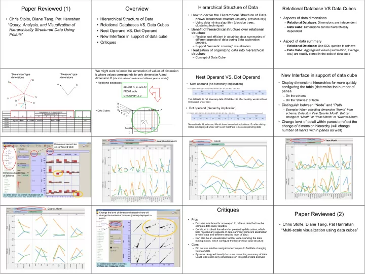
Dimension hierarchies
- n configured table
Dimension hierarchies
- n schema
Year.Quarter.Month Month Year.Month Quarter.Month Change the level of dimension hierarchy here will change the number of datasets (marks) displayed in panes
Critiques
- Pros
– Provides interfaces for non-expert to retrieve data that involve complex data query algebra – Construct a robust formalism for presenting data cubes, which help reveal many aspects of data summary (different abstraction level of data and different detailed level of data) – Can also be an visualization tool for understanding the data mining model, which configure the hierarchical data structure.
- Cons
– Did not use intuitive navigation techniques to facilitate changing views of data – Systems designed heavily focus on presenting summary of data. Could lead users only concentrate on this part of data analysis
Paper Reviewed (2)
- Chris Stolte, Diane Tang, Pat Hanrahan