Pairwise alignment using HMMs - Ch.4 Durbin et al. Recall the - - PowerPoint PPT Presentation

1

Pairwise alignment using HMMs - Ch.4 Durbin et al.

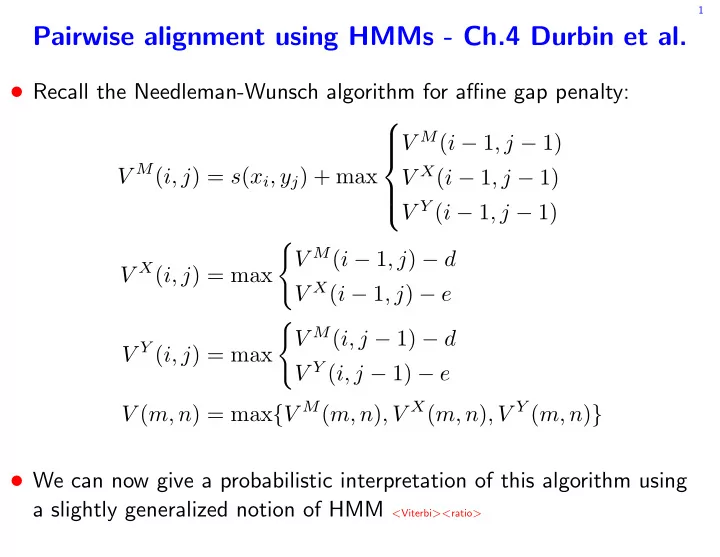
• Recall the Needleman-Wunsch algorithm for affine gap penalty:

V M(i, j) = s(xi, yj) + max        V M(i − 1, j − 1) V X(i − 1, j − 1) V Y (i − 1, j − 1) V X(i, j) = max

• V M(i − 1, j) − d

V X(i − 1, j) − e V Y (i, j) = max

• V M(i, j − 1) − d

V Y (i, j − 1) − e V (m, n) = max{V M(m, n), V X(m, n), V Y (m, n)}

• We can now give a probabilistic interpretation of this algorithm using

a slightly generalized notion of HMM <Viterbi><ratio>

2

“Pair HMMs”

• A pair HMM generates an alignment by simultaneously producing two

sequences of symbols

• The M (match) state emits a pair of symbols, one for each sequence:

(xi, yj) ∼ p(xi, yj)

• The X (x-insertion) state emits only an “X symbol”: xi ∼ q(xi)
• The Y (y-insertion) state emits only a “Y symbol”: yj ∼ q(yj)

3

Pair HMM - cont.

• The model above does not generate a probability distribution over all

possible sequences

• for that we need to add Begin and End states:
• The expected length of the generated alignment is 1

τ

• The transitions of the Markov chain are given by pMM = pBM =

1 − 2δ − τ, pMX = pMY = δ, pXX = ε, pXM = 1 − ε − δ, etc.

4

Most probable alignment

• We can only observe x and y: unlike in HMMs we cannot observe the

joint emission from the M state

• Let Sij be the set of paths s compatible with an alignment of x1:i

and y1:j

• i.e.

the path visits states {M, X} exatly i times and states {M, Y } exatly j times

• Given the observed sequences x and y, Smn is in 1:1 correspondence

with the set of alignments of x and y

• The advantage of the pair HMM framework is now we can ask for the

most probable alignment given the data

• same as maximizing p(x, y, s) over the path s

5

Most probable alignment - cont.

• For α ∈ {M, X, Y } let

vα(i, j) = max

s∈Sij:s(|s|)=α p(x1:i, y1:j, s1:|s|),

where |s| is the length of the alignment of s.

• Clearly,

max

s

p(x, y, s) = max{vM(m, n), vX(m, n), vY (m, n)} · τ

• note that the rhs is in fact vE(m, n)
• The following claim shows how to recursively compute vα(i, j)

6

Viterbi for pair HMM

• Claim. For m ≥ i ≥ 0, n ≥ j ≥ 0 with i + j > 0:

vM(i, j) = p(xi, yj) · max        pMM · vM(i − 1, j − 1) pXM · vX(i − 1, j − 1) pY M · vY (i − 1, j − 1) vX(i, j) = q(xi) · max

• pMX · vM(i − 1, j)

pXX · vX(i − 1, j) vY (i, j) = q(yj) · max

• pMY · vM(i, j − 1)

pY Y · vY (i, j − 1) where v•(i, −1) = v•(−1, j) = v[XY ](0, 0) = 0, and vM(0, 0) := 1

• vM(0, 0) is in fact a surrogate for vB(0, 0)

<Needleman-Wunsch><ratio>

7

Viterbi for pair HMM - cont.

• This algorithm is similar but still differs from Needleman-Wunsch
• logarithms should be used
• log-odds

ratio rather than log-odds are computed (BLOSUM/PAM)

• The following random model simply dumps the symbols of x and the

y without any correlation (no match states) pR(x, y) = η(1 − η)m

m

• i=1

q(xi)η(1 − η)n

n

• j=1

q(yj)

8

Viterbi for maximal log-odds ratio

• Look for the path s that maximizes the log-odds ratio log pM(s,x,y)

pR(s,x,y)

• Let V α(i, j) = maxs∈Sij:s(|s|)=α log

pM(x1:i,y1:j,s1:|s|) pR(x1:i,y1:j,s1:|s|)

• Analogously to the log-odds case we have

V M(i, j) = log p(xi, yj) q(xi)q(yj) + max          log pMM

(1−η)2 + V M(i − 1, j − 1)

log

pXM (1−η)2 + V X(i − 1, j − 1)

log

pY M (1−η)2 + V Y (i − 1, j − 1)

V X(i, j) = log q(xi) q(xi) + max

• log pMX

1−η + V M(i − 1, j)

log pXX

1−η + V X(i − 1, j)

V Y (i, j) = log q(yj) q(yj) + max

• log pMY

1−η + V M(i, j − 1)

log pY Y

1−η + V Y (i, j − 1)

<Needleman-Wunsch>

9

Viterbi as Needleman-Wunsch

• To see the equivalence more clearly it is convenient to introduce

s(a, b) = log p(a, b) q(a)q(b) + log pMM (1 − η)2 −d = log pMX/Y (1 − η) + log pX/Y M pMM −e = log pXX/Y Y 1 − η

• s(a, b) “assumes” we come from M
• d “pre-corrects” that by adding c := log

pX/Y M pMM

• Only η2 and the transitions from X/Y to E are left unbalanced:

V M(0, 0) := −2 log η V E(m, n) := max{V M(m, n), V X(m, n) − c, V Y (m, n) − c}

10

pair HMM for local alignment

• As before we can look for optimal log-odds or log-odds ratio paths

(the latter case will yield Smith-Waterman)

11

The likelihood that x and y are aligned

• While it is interesting to note that the Needleman-Wunsch algorithm

can be cast in the language of HMM

• The real power of the HMM framework is that it allows us to answer

questions such as

• what is the likelihood that x and y are aligned, i.e., that they

were generated by the model?

• The answer is the probability that x, y will be generated by the model

p(x, y) =

s p(x, y, s)

• An analogue of the forward algorithm computes that: let

f α(i, j) := P(X1:i = x1:i, Y 1:j = y1:j, S(τij) = α), where τij := min{k :

k

• l=1

1S(l)∈{M,X} = i and

k

• l=1

1S(l)∈{M,Y } = j}

12

The likelihood that x and y are aligned - cont.

• Claim. With the initial conditions

f M(0, 0) = 1 f [XY ](0, 0) = 0 f •(i, −1) = f •(−1, j) = 0, for i ≥ 0, j ≥ 0 with i + j > 0: f M(i, j) = p(xi, yj)[pMM · f M(i − 1, j − 1) + pXM · f X(i − 1, j − 1) + pY M · f Y (i − 1, j − 1)] f X(i, j) = q(xi)[pMX · f M(i − 1, j) + pXX · f X(i − 1, j)] f Y (i, j) = q(yj)[pMY · f M(i, j − 1) + pY Y · f Y (i, j − 1)], and p(x, y) = f E(m, n) = τ[f M(m, n) + f X(m, n) + f Y (m, n)]

13

Posterior distribution of an alignment

• With p(x, y) we can find the posterior distribution of any particular

alignment s: p(s|x, y) = p(x,y,s)

p(x,y)

• In particular we can apply it for s∗, the Viterbi solution
• The answer is typically depressingly small

⊲ For example in the alpha globing vs. leghemoglobin case: ⊲ p(s∗|x, y) = 4.6 × 10−6

14

Sampling from the posterior distribution

• Given the poor posterior probability of the Viterbi alignment
• are there parts of the alignment which we are more confident of?
• can we estimate posterior expectation of functionals of the align-

ment as in posterior decoding?

• We can do that through MC sampling from the posterior distribution
• backward sampling (using forward algorithm)
• forward sampling (using backward algorithm)

15

The backward algorithm

• Analogously to the backward function for HMMs we define

bα(i, j) := P(Xi+1:m = xi+1:m, Y j+1:n = yj+1:n, S(τij) = α), where τij := min{k :

k

• l=1

1S(l)∈{M,X} = i and

k

• l=1

1S(l)∈{M,Y } = j}

• Durbin et al.:
• as before we can add bM(0, 0) as a surrogate for bB(0, 0)

16

Forward posterior sampling (backward algorithm)

• Inductively draw from the posterior distribution as follows:
• start at state B with (i, j) := (0, 0)
• while (i, j) = (m, n):

⊲ given our hitherto path s ∈ S(i, j) randomly choose our

next state α according to P[S(|s| + 1) = α|x, y, s]

⊲ update: s = s ∧ α, and

(i, j) := (i+(α), j+(α)) := (i + 1α∈{M,X}, j + 1α∈{M,Y })

• output the resulting s ∈ S(m, n) (why is s ∈ S(m, n)?)
• Claim. The probability that we draw a path s ∈ S(m, n) is p(s|x, y)
• Proof. To simplify notations assume s(0) = B does not count toward

|s|. Then p(s|x, y) =

|s|

• i=1

p(s(i)|x, y, s0:i−1)

17

Forward posterior sampling - cont.

• The algorithm hinges on finding

P[S(|s| + 1) = α|x, y, s] = p(s ∧ α, x, y) p(s, x, y)

• Using the properties of the HMM we have:

p(s ∧ α, x, y) = p(x1:i, y1:j, s) × P[S(|s| + 1) = α, x(i+(α)), y(j+(α))|xi, yj, s] × p[xi+(α)+1:m, yj+(α)+1:n|S(|s| + 1) = α] P[S(|s| + 1) = α, x(i+(α)), y(j+(α))|xi, yj, s] =        ps(|s|),M · p(x(i + 1), y(j + 1)) α = M ps(|s|),X · q(x(i + 1)) α = X ps(|s|),Y · q(y(j + 1)) α = Y

18

• Note that

p[xi+(α)+1:m, yj+(α)+1:n|S(|s| + 1) = α] = bα(i+(α), j+(α))

• Finally,

p(s, x, y) = p(x1:i, y1:j, s)p(xi+1:m, yj+1:n|s) = p(x1:i, y1:j, s)bs(|s|)(i, j) Thus, P[S(|s| + 1) = α|x, y, s] = bα(i+(α), j+(α)) bs(|s|)(i, j) ×        ps(|s|),M · p(x(i + 1), y(j + 1)) α = M ps(|s|),X · q(x(i + 1)) α = X ps(|s|),Y · q(y(j + 1)) α = Y

19

Posterior probability that xi is aligned to yj

• We can estimate the posterior probability that xi is aligned to yj by

posterior sampling of alignments

• but we can also compute it directly

⊲ analogous to computing P(S(i) = k|x) for HMMs

• Let Xi ⋄ Yj denote the event Xi is aligned to Yj, then

P(X = x, Y = y, Xi ⋄ Yj) = P(X1:i = x1:i, Y 1:j = y1:j, S(τij) = M) × P[Xi+1:m = xi+1:m, Y j+1:n = yj+1:n|S(τij) = M] = f M(i, j)bM(i, j) therefore P(Xi ⋄ Yj|X = x, Y = y) = f M(i, j)bM(i, j) p(x, y) = f M(i, j)bM(i, j) f E(m, n)

20

Optimizing for the “expected accuracy”

• An intuitively appealing measure of the accuracy of s is

A(s) =

• Mij∈s

p(xi ⋄ yj|x, y)

• A(s) is the expected overlap in M states between s and a

random alignment drawn according to the posterior distribution

• Finding a path s which maximizes A(s) is easy: let A(i, j) be the
• ptimal accuracy we can gain using only x1:i and y1:j

A(i, j) = max        A(i − 1, j − 1) + p(xi ⋄ yj|x, y) A(i − 1, j) A(i, j − 1)

21

Viterbi failure

• Can the Viterbi algorithm discriminate between data generated by the

following model vs. the random one?

• Maximizing the log-likelihood or llr is equivalent here
• If α4q(a)q(b)q(a)q(c) > 1 − α then pS(abac) > pB(abac) and the

Viterbi path will never visit state B

• Since state S is random, the Viterbi path cannot discriminate between

the model and random data

22

Viterbi failure - cont.

• However, if the data is long enough clearly the model is distinguishable

from random:

• fo(abac) → pM(abac) > pS(abac)
• so simply observing the frequency of abac should work for suffi-

ciently long sequences

• Maximizing the likelihood is not always the appropriate approach
• However, comparing pM(x) and pR(x) should discriminate the two

models

• as this is the optimal test and we just saw we can discriminate
• Bonus points: figure out Figure 4.8