Pairs Design Pattern map(docID a, doc d) for all term w in doc d do - - PDF document

10/14/2011 1

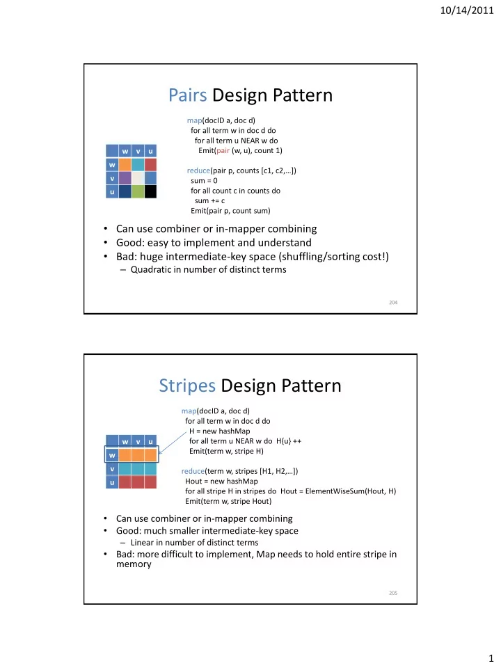
Pairs Design Pattern

• Can use combiner or in-mapper combining
• Good: easy to implement and understand
• Bad: huge intermediate-key space (shuffling/sorting cost!)

– Quadratic in number of distinct terms

204

map(docID a, doc d) for all term w in doc d do for all term u NEAR w do Emit(pair (w, u), count 1) reduce(pair p, counts [c1, c2,…]) sum = 0 for all count c in counts do sum += c Emit(pair p, count sum) w v u w v u

Stripes Design Pattern

• Can use combiner or in-mapper combining
• Good: much smaller intermediate-key space

– Linear in number of distinct terms

• Bad: more difficult to implement, Map needs to hold entire stripe in

memory

205

map(docID a, doc d) for all term w in doc d do H = new hashMap for all term u NEAR w do H{u} ++ Emit(term w, stripe H) reduce(term w, stripes [H1, H2,…]) Hout = new hashMap for all stripe H in stripes do Hout = ElementWiseSum(Hout, H) Emit(term w, stripe Hout) w v u w v u

10/14/2011 2

Beyond Pairs and Stripes

• In general, it is not clear which approach is better

– Some experiments indicate stripes win for co-

• ccurrence matrix computation
• Pairs and stripes are special cases of shapes for

covering the entire matrix

– Could use sub-stripes, or partition matrix horizontally and vertically into more square-like shapes etc.

• Can also be applied to higher-dimensional arrays
• Will see interesting version of this idea for joins

206

(3) Relative Frequencies

• Important for data mining
• E.g., for each species and color, compute

probability of color for that species

– Probability of Northern Cardinal being red, P(color = red | species = N.C.)

• Count f(N.C.), the frequency of observations for N.C.

(marginal)

• Count f(N.C., red), the frequency of observations for red

N.C.’s (joint event)

• P(red | N.C.) = f(N.C., red) / f(N.C.)
• Similarly: normalize word co-occurrence vector

for word w by dividing it by w’s frequency

207

10/14/2011 3

Bird Probabilities Using Stripes

• Use species as intermediate key

– One stripe per species, e.g., stripe[N.C.]

• (stripe[species])[color] stores f(species, color)
• Map: for each observation of (species S, color C) in an
• bservation event, increment (stripe[S])[C]

– Output (S, stripe[S])

• Reduce: for each species S, add all stripes for S

– Result: stripeSum[S] with total counts for each color for S – Can get f(S) by adding all stripeSum[S] values together – Get probability P(color = C | species = S) as (stripeSum[S])[C] / f(S)

208

Discussion, Part 1

• Stripe is great fit for relative frequency

computation

• All values for computing the final result are in

the stripe

• Any smaller unit would miss some of the joint

events needed for computing f(S), the marginal for the species

• So, this would be a problem for the pairs

pattern

209

10/14/2011 4

Bird Probabilities Using Pairs

• Intermediate key is (species, color)
• Map produces partial counts for each species-

color combination in input

• Reduce can compute f(species, color), the

total count of each species-color combination

• But: cannot compute marginal f(S)

– Reduce needs to sum f(S, color) for all colors for species S

210

Pairs-Based Solution, Take 1

• Make sure all values f(S, color) for the same

species end up in the same reduce task

– Define custom partitioning function on species

• Maintain state across different keys in same

reduce task

• This essentially simulates the stripes approach

in the reduce task, creating big reduce tasks when there are many colors

• Can we do better?

211

10/14/2011 5

Discussion, Part 2

• Pairs-based algorithm would work better, if

marginal f(S) was known already

– Reducer computes f(species, color) and then outputs f(species, color) / f(species)

• We can compute the species marginals f(species)

in a separate MapReduce job first

• Better: fold this into a single MapReduce job

– Problem: easy to compute f(S) from all f(S, color), but how do we compute f(S) before knowing f(S, color)?

212

Bird Probabilities Using Pairs, Take 2

• Map: for each observation event, emit ((species S, color C),

1) and ((species S, dummyColor), 1) for each species-color combination encountered

• Use custom partitioner that partitions based on the species

component only

• Use custom key comparator such that (S, dummyColor) is

before all (S, C) for real colors C

– Reducer computes f(S) before the f(S, C)

• Reducer keeps f(S) in state for duration of entire task

– Reducer then computes f(S, C) for each C, outputting f(S, C) / f(S)

• Advantage: avoids having to manage all colors for a species

together

213

10/14/2011 6

Order Inversion Design Pattern

• Occurs surprisingly often during data analysis
• Solution 1: use complex data structures that bring the

right results together

– Array structure used by stripes pattern

• Solution 2: turn synchronization into ordering problem

– Key sort order enforces computation order – Partitioner for key space assigns appropriate partial results to each reduce task – Reducer maintains task-level state across Reduce invocations – Works for simpler pairs pattern, which uses simpler data structures and requires less reducer memory

214

(4) Secondary Sorting

• Recall the weather data: for simplicity assume
• bservations are (date, stationID, temperature)
• Goal: for each station, create a time series of

temperature measurements

• Per-station data: use stationID as intermediate

key

• Problem: reducers receive huge number of (date,

temp) pairs for each station

– Have to be sorted by user code

215

10/14/2011 7

Can Hadoop Do The Sorting?

• Use (stationID, date) as intermediate key

– Problem: records for the some station might end up in different reduce tasks – Solution: custom partitioner, using only stationID component of key for partitioning

• General value-to-key conversion design pattern

– To partition by X and then sort each X-group by Y, make (X, Y) the key – Define key comparator to order by composite key (X, Y) – Define partitioner and grouping comparator for (X, Y) to consider only X for partitioning and grouping

• Grouping part is necessary if all dates for a station should be

processed in the same Reduce invocation (otherwise each station- date combination ends up in a different Reduce invocation)

216

Design Pattern Summary

• In-mapper combining: do work of combiner in

mapper

• Pairs and stripes: for keeping track of joint

events

• Order inversion: convert sequencing of

computation into sorting problem

• Value-to-key conversion: scalable solution for

secondary sorting, without writing own sort code

217

10/14/2011 8

Tools for Synchronization

• Cleverly-constructed data structures for key

and values to bring data together

• Preserving state in mappers and reducers,

together with capability to add initialization and termination code for entire task

• Sort order of intermediate keys to control
• rder in which reducers process keys
• Custom partitioner to control which reducer

processes which keys

218

Issues and Tradeoffs

• Number of key-value pairs

– Object creation overhead – Time for sorting and shuffling pairs across the network

• Size of each key-value pair

– (De-)serialization overhead

• Local aggregation

– Opportunities to perform local aggregation vary – Combiners can make a big difference – Combiners vs. in-mapper combining – RAM vs. disk vs. network

219

10/14/2011 9

220

Now that we have seen important design patterns and MapReduce algorithms for simpler problems, let’s look at some more complex problems.

Joins in MapReduce

• Data sets S={s1,..., s|S|} and T={t1,..., t|T|}
• Find all pairs (si, tj) that satisfy some predicate
• Examples

– Pairs of similar or complementary function summaries – Facebook and Twitter posts by same user or from same location

• Typical goal: minimize job completion time

221

10/14/2011 10

Function-Join Pattern

• Find groups of summaries with certain properties
• f interest

– Similar trends, opposite trends, correlations – Groups not known a priori, need to be discovered

222

Existing Join Support

• Hadoop has some built-in join support, but
• ur goal is to design our own algorithms

– Built-in support is limited – We want to understand important algorithm design principles

• “Join” usually just means equi-join, but we

also want to support other join predicates

• Note: recall join discussion from earlier lecture

223

10/14/2011 11

Joining Large With Small

• Assume data set T is small enough to fit in

memory

• Can run Map-only join

– Load T onto every mapper – Map: join incoming S-tuple with T, output all matching pairs

• Can scan entire T (nested loop) or use index on T (index

nested loop)

• Downside: need to copy T to all mappers

– Not so bad, since T is small

224

Distributed Cache

• Efficient way to copy files to all nodes

processing a certain task

– Use it to send small T to all mappers

• Part of the job configuration
• Hadoop still needs to move the data to the

worker nodes, so use this with care

– But it avoids copying the file for every task on the same node

225

10/14/2011 12

DFS nodes Transfer Input Map Transfer Map Output Reduce Transfer Reduce Output list(v3) list(k2,v2) (k2,list(v2)) (k1,v1) DFS nodes Mappers Reducers

Recall: Standard Equi-Join Algorithm

• Join condition: S.A=T.A
• Map(s) = (s.A, s); Map(t) = (t.A, t)
• Reduce combines S-tuples and T-tuples with same key

226

s1,1 s1,1 1,(s1,1) s5,1 s5,1 1,(s5,1) 1,(t3,1) t3,1 t3,1 t8,1 t8,1 1,(t8,1) 1,[(s5,1)(t3,1)(s1,1)(t8,1)] (s5,t3) (s1,t3) (s1,t8) (s5,t8) s3,2 t1,2 s3,2 t1,2 2,[(s3,2)(t1,2)] (s3,t1) 2,(t1,2) 2,(s3,2)

Problems With Standard Approach

• Degree of parallelism limited by number of

distinct A-values

• Data skew

– If one A-value dominates, reducer processing that key will become bottleneck

• Does not generalize to other joins

227

10/14/2011 13

Reducer-Centric Cost Model

• Difference between join implementations starts

with Map output

228

Join output time=f(input size) time=f(output size)

• utput

Sort input by key Read input algorithm Send join

• utput

Receive Mapper Run join Reducer Mapper output

Optimization Goal: Minimal Job Completion time

• Assume all reducers are similarly capable
• Processing time at reducer is approximately

monotonic in input and output size

• Hence need to minimize:

– Max-reducer-input and/or – Max-reducer-output

• Join problem classification

– Input-size dominated: minimize max-reducer-input – Output-size dominated: minimize max-reducer-output – Input-output balanced: minimize combination of both

229

10/14/2011 14

Join Model

• Join-matrix M: M(i, j) = true, if and only if (si, tj) in join

result

• Cover each true-valued cell by exactly one reducer

230

M(2,5) S 5 7 7 7 8 9 7 5 7 8 9 9 T S.A = T.A S 5 7 7 7 8 9 7 5 7 8 9 9 T abs(S.A - T.A) < 2 S 5 7 7 7 8 9 7 5 7 8 9 9 T S.A >= T.A M(2,1)

231

5 7 8 9 3 3 3 2 2 1 1 1 1 2 3 2 1 Input: S2,S3,S4,S6 T3,T4,T5,T6 Output: 4 tuples Input: S2,S3,S5 T2,T4,T6 Output: 3 tuples R3: key 3 Input: S1,S2,S3 T1,T2,T3 Output: 3 tuples max-reducer-input = 8 R1: key 1 R2: key 2 max-reducer-output = 4 S1,S4 T1,T5 2 tuples Input: S2,S3 T2,T3,T4 Output: 6 tuples R3: key 9 Input: S5,S6 T6 Output: 2 tuples R2: key 7 R1: keys 5,8 Output: Input: max-reducer-input = 5 max-reducer-output = 6 R1: key 1 Input: S1,S2,S3 T1,T2 Output: 3 tuples Input: S2,S3 T3,T4 Output: 4 tuples R3: key 3 Input: S4,S5,S6 T5,T6 Output: 3 tuples max-reducer-input = 5 max-reducer-output = 4 R2: key 2 S 5 7 7 7 8 9 7 5 7 8 9 9 T S 5 7 7 7 8 9 7 5 7 8 9 9 T S 5 7 7 7 8 9 7 5 7 8 9 9 T key

Standard Equi-Join Alg.: Random Assignment: Balanced Algorithm: