Ozone Conceptual Model for the Killeen-Temple-Fort Hood Area CTCOG - - PowerPoint PPT Presentation

Template Template

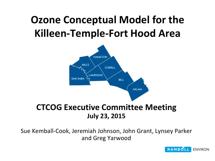
Ozone Conceptual Model for the Killeen-Temple-Fort Hood Area

CTCOG Executive Committee Meeting

July 23, 2015

Sue Kemball-Cook, Jeremiah Johnson, John Grant, Lynsey Parker and Greg Yarwood

Ozone

Figure: http://esrl.noaa.gov/csd/assessments/ozone/2006/chapters/Q1.pdf

2

“Good up high, bad nearby”

3

Ground Level Ozone and Air Quality

• Ozone is the main ingredient

in smog

– Affects human lung function (asthma, bronchitis) – Damages vegetation

• Clean Air Act primary

standard for ozone (NAAQS)

– Based on health impacts for sensitive groups – Economic penalties for non- attainment

• Forms from NOx and VOC in

presence of sunlight, not emitted directly

Figures:US EPA http://www.epa.gov/air/ozonepollution/basic.html

Conceptual Model

4

• What factors

contribute to high

• zone in the KTF area?

– Emission inventory – Ozone and weather data and trends – Photochemical modeling

Ozone Trends at Killeen

5

KTF Area Emission Inventory Review

• TCEQ develops

inventory for the State of Texas

• NNAs review the

TCEQ EI for their area

• Identify emissions

sources that are:

– Uncertain, – Over- or under- estimated – Could be improved with local data

6

CTCOG figure: http://ctcog.org/

Emission Inventory

• List of sources of air emissions of ozone precursors

– Point Sources

• Emissions sources that meet TCEQ thresholds for reporting
• Usually emitted from a stack
• Power plants, chemical plants, compressor stations, etc.

– Non-Point Emissions Sources

• On-road mobile (cars, trucks, buses, motorcycles)
• Off-road mobile (locomotives, drill rigs, construction, ag

equipment)

• Area sources (dry cleaners, degreasing operations, wells)
• Biogenics (trees, crops, microbes in soil, fertilizer application)

7

Summary of KTF Area 2012 Emission Inventory

• Mobile sources are more than 50% of NOx inventory

– Substantial biogenic NOx emissions contribution – agriculture?

• VOC inventory dominated by biogenics (natural sources)

– Abundant biogenics mean there is typically sufficient VOC to form ozone

• Ozone formation limited by the amount of available NOx

8

Total NOx Emissions: 62 tpd Total VOC Emissions: 1,026 tpd

Anthropogenic Emissions by County

• 78% of NOx emissions from Bell and Milam Counties
• Nearly all of Milam Point source NOx emissions are from Sandow Power

Plant

• Bell County NOx mainly due to on-road mobile (I-35)
• Milam area source VOC emissions mainly due to oil and gas
• Bell County off-road due to locomotives, ag, construction and mining

9

Off-Road NOx Emissions Sources by County

• Largest off-road

categories are locomotives, ag, construction and mining

10

2012 KTF Area NOx Point Sources

11

Panda Temple Power Plant not shown

Panda Temple Power Plant

• Built in two phases, both
• perational by end of 2015
• 4 combined cycle natural

gas-fired combustion turbines

• DLN + SCR NOx emission

controls

• Baseload/peaking units

– Likely to be operating on high

• zone days
• New source of NOx near

monitor and not in TCEQ 2012 emission inventory

12

Panda Power Plant Temple Georgia Monitor 8 miles

Area Source NOx Emissions by County

• Oil and gas NOx from

artificial lift engines, heaters and gas compressor engines

13

Area Source VOC Emissions by County

• Non-O&G area VOC emissions

from a variety of sources

14

O&G

15

Weather Conditions Associated with High Ozone at the Killeen Monitor

• Strong sunlight (April-October, clear/partly sunny skies)
• High temperatures (T > 82°F)
• Light winds (< 12 mph)
• Winds coming from north-southwesterly direction

– Transport of polluted, continental air – Low ozone days have strong, southerly winds that bring clean maritime air from Gulf of Mexico

• High pressure system, stationary front, or cold front

passage

Photochemical Modeling

• Ozone model (photochemical grid model) is a

computer simulation of the atmosphere

• Use the model to understand the area’s ozone

problem and suggest methods to reduce ozone

• Determine how much of the ozone at a given location

can be attributed to:

– Local emissions – Transport from other parts of Texas, other States, and from outside North America

• Determine how much of an area’s ozone can be

reduced by NOx vs. VOC emissions reductions

16

Ozone Model

17

AWMA Environmental Manager magazine July 2012 issue on AQMEII Douw Steyn, Peter Builtjes , Martijn Schaap and Greg Yarwood

Receptor Y Source Region X How do ozone, NOx, VOC, etc. change with time?

2012 Model Performance at Killeen

18

June 2012 Ozone Source Apportionment for Killeen Monitor

• Transported ozone dominates local contribution
• Local contribution from KTF is affected by uncertainties in KTF emission

inventory, but modeling results indicate it can exceed 10 ppb

– Local emissions controls can potentially reduce ozone at Killeen but cannot eliminate the ozone problem

19

KTF Area (non-KTF Area)

Ozone Impact of KTF Emissions vs. Transport

• Contribution of transport is far larger than local

contribution from KTF emissions during June 2012

20

Temple Killeen

Maximum Contribution of KTF Area Emissions to Ozone at Killeen and Temple

• Ozone formation in KTF area is NOx-limited

– Consistent with emission inventory VOC/NOx ratio

• Local emissions controls should focus on NOx reductions

21

Temple Killeen

• Consistent with emission inventory

22

• Results similar to Killeen monitor, but higher contribution from elevated

points

– Larger influence of Sandow power plant

23

Summary

• Ambient monitoring data and ozone modeling show the

importance of transport in determining ozone levels at the Killeen monitor

– Local emissions make a far smaller but non-zero contribution to Killeen ozone – Magnitude of local ozone contribution affected by uncertainty in emission inventory

• Biogenic VOC emissions are sufficiently high that ozone

formation is generally NOx-limited

– Potential ozone impact of KTF emissions determined by NOx emissions

• Local emissions control strategies aimed at reducing local

contributions to KTF area ozone should focus on reducing NOx emissions

24

Recommendations for FY16-17 Technical Work

• Analyze and rank potential local NOx emission

control strategies

• Refine TCEQ 2012 emission inventory for KTF area
• Photochemical modeling

– Diagnose and improve 2012 TCEQ ozone model performance on high ozone days at Killeen – Evaluate emissions and potential ozone impacts of Panda Temple Power Plant – Evaluate ozone impacts of emission control strategies

• Analyze 2016-2017 high ozone days at Killeen and

Temple Georgia

25

END

26

Regional Design Value Trends

27

Oil and Gas Well Count Trends

• Most of the oil and gas wells in the 7-county area are

located in Milam County

• Sharp increase in well counts since 2012
• Oil wells far outnumber gas wells

28

Active Gas Wells

KTF Area Production Trends

• Sharp increase in oil

production in 2012

• Production trends seem

inconsistent with well counts (e.g. 2012 and 2014)

– 2014 Railroad Commission production data may be incomplete

29

Condensate (bbl/yr) Active Gas Well Count

The Eagle Ford Shale

• The Eagle

Ford Shale extends into Milam County

• Milam Eagle

Ford well count is very small as of March, 2015

30

Railroads

• Emissions distribution consistent with rail line locations

31

Killeen Monitor Wind Roses

• On MDA8 ≤ 60 ppb days, stronger, southeasterly winds
• On MDA8 > 75 ppb days, lighter northeasterly through

southeasterly winds

32

MDA8 ≤ 60 ppb MDA8 > 75 ppb

Killeen Monitor Wind Roses

• On MDA8 ≤ 60 ppb days, stronger, southeasterly winds
• On MDA8 > 70 ppb days, lighter northeasterly through

southwesterly winds

33

MDA8 ≤ 60 ppb MDA8 > 70 ppb

HYSPLIT Model 24-Hour Back Trajectories

• When MDA8 ≤ 60 ppb, back trajectories are longer (higher wind speed) and most

frequently extend southward

• When MDA8 >75 ppb back trajectories are shorter (lower wind speed) and most

frequently extend northeastward

34

HYSPLIT Model 24-Hour Back Trajectories

• When MDA8 ≤ 60 ppb, back trajectories are longer (higher wind speed) and most

frequently extend southward

• When MDA8 >70 ppb back trajectories are shorter (lower wind speed) and most

frequently extend northeast through southwest

35

Regional NOx Emissions

• Texas areas with higher NOx emissions to the North

through southwest

36

CAMx Source Apportionment Map

37

Ozone Contributions from Surrounding Regions

38

High Ozone Day Analysis

• Ozone at local and regional

monitors

• Winds, origin of air mass
• Relative importance of

transport and local emissions

39