overview kursus 02402 introduction to statistics
play

Overview Kursus 02402 Introduction to Statistics Oneway analysis - PowerPoint PPT Presentation

Overview Kursus 02402 Introduction to Statistics Oneway analysis of Variance (ANOVA) 1 Intro Example Lecture 12: Analysis of Variance Model and hypothesis Computation - decomposition of variance and the ANOVA table Test, F-distributions


  1. Overview Kursus 02402 Introduction to Statistics Oneway analysis of Variance (ANOVA) 1 Intro Example Lecture 12: Analysis of Variance Model and hypothesis Computation - decomposition of variance and the ANOVA table Test, F-distributions Example 1 Per Bruun Brockhoff Post hoc comparisons Two-way ANOVA DTU Informatics 2 Example 2 Building 305 - room 110 Danish Technical University Model and variance decomposition 2800 Lyngby – Denmark The ANOVA Table e-mail: pbb@imm.dtu.dk Example 2 R (R note 11) 3 Per Bruun Brockhoff (pbb@imm.dtu.dk) Introduction to Statistics, Lecture 12 Fall 2012 1 / 36 Per Bruun Brockhoff (pbb@imm.dtu.dk) Introduction to Statistics, Lecture 12 Fall 2012 2 / 36 Oneway analysis of Variance (ANOVA) Intro Example
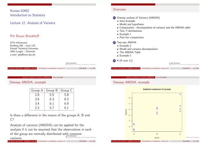
 Oneway analysis of Variance (ANOVA) Intro Example Oneway ANOVA, example Oneway ANOVA, example Graphical comparison of 3 groups Group A Group B Group C 2.8 5.5 5.8 3.6 6.3 8.3 8 3.4 6.1 6.9 7 2.3 5.7 6.1 response 6 Is there a difference in the means of the groups A, B and 5 C? 4 Analysis of variance (ANOVA) can be applied for the 3 analysis if it can be assumed that the observations in each of the group are normally distributed with constant A B C variance. groups Per Bruun Brockhoff (pbb@imm.dtu.dk) Introduction to Statistics, Lecture 12 Fall 2012 4 / 36 Per Bruun Brockhoff (pbb@imm.dtu.dk) Introduction to Statistics, Lecture 12 Fall 2012 5 / 36

  2. Oneway analysis of Variance (ANOVA) Intro Example Oneway analysis of Variance (ANOVA) Intro Example Oneway ANOVA, example Oneway ANOVA, example Per Bruun Brockhoff (pbb@imm.dtu.dk) Introduction to Statistics, Lecture 12 Fall 2012 6 / 36 Per Bruun Brockhoff (pbb@imm.dtu.dk) Introduction to Statistics, Lecture 12 Fall 2012 7 / 36 Oneway analysis of Variance (ANOVA) Model and hypothesis Oneway analysis of Variance (ANOVA) Model and hypothesis One-Way ANOVA, the model One-Way ANOVA, the hypothesis We consider the model We want to compare (more than two) means µ + α i in the model Y ij = µ + α i + ǫ ij ǫ ij ∼ N (0 , σ 2 ) Y ij = µ + α i + ǫ ij , where it is assumed that that is, we can formulate the hypotheses: ǫ ij ∼ N (0 , σ 2 ) H 0 : α i = 0 for all i H 1 : α i � = 0 for at least one i µ is the mean of all the observations α i gives the level of ’group’ i Per Bruun Brockhoff (pbb@imm.dtu.dk) Introduction to Statistics, Lecture 12 Fall 2012 8 / 36 Per Bruun Brockhoff (pbb@imm.dtu.dk) Introduction to Statistics, Lecture 12 Fall 2012 9 / 36

  3. Computation - decomposition of variance and the ANOVA Computation - decomposition of variance and the ANOVA Oneway analysis of Variance (ANOVA) table Oneway analysis of Variance (ANOVA) table One-Way ANOVA, the decomposition Formulas for Sums of Squares Corresponding to the model k n i � � y 2 ǫ ij ∼ N (0 , σ 2 ) SST = ij − C Y ij = µ + α i + ǫ ij , i =1 j =1 the total variation in the data can be R note it up into: k T 2 � i SS ( Tr ) = − C SST = SS ( Tr ) + SSE n i i =1 ’One-way’ means that we only have one factor on k levels where n i k to examine. C = T 2 . � � T i = y ij T . = T i The method is called analysis of variance, since the tests N j =1 i =1 are carried out by comparing variances. Per Bruun Brockhoff (pbb@imm.dtu.dk) Introduction to Statistics, Lecture 12 Fall 2012 10 / 36 Per Bruun Brockhoff (pbb@imm.dtu.dk) Introduction to Statistics, Lecture 12 Fall 2012 11 / 36 Computation - decomposition of variance and the ANOVA Oneway analysis of Variance (ANOVA) table Oneway analysis of Variance (ANOVA) Test, F-distributions The ANOVA Table One-Way ANOVA, the F-test We have: Source of Degrees of Sums of Test- SST = SS ( Tr ) + SSE variation freedom squares statistic F and the test statistic, F : SS ( Tr ) / ( k − 1) Treatment k − 1 SS ( Tr ) SSE/ ( N − k ) F = SS ( Tr ) / ( k − 1) Residual N-k SSE SSE/ ( N − k ) Total N-1 SST where k is the number of levels of the factor and N is the total number of observations. Per Bruun Brockhoff (pbb@imm.dtu.dk) Introduction to Statistics, Lecture 12 Fall 2012 12 / 36 Per Bruun Brockhoff (pbb@imm.dtu.dk) Introduction to Statistics, Lecture 12 Fall 2012 13 / 36

  4. Oneway analysis of Variance (ANOVA) Test, F-distributions Oneway analysis of Variance (ANOVA) Test, F-distributions One-Way ANOVA, test F-distributions Example of a F−distribution The test statistic F is calculated and the level of significance α chosen 0.6 F = SS ( Tr ) / ( k − 1) 0.4 density SSE/ ( N − k ) The test statistic is compared to a quantile in the F 0.2 distribution: F ∼ F α ( k − 1 , N − k ) 0.0 0 1 2 3 4 5 6 x Per Bruun Brockhoff (pbb@imm.dtu.dk) Introduction to Statistics, Lecture 12 Fall 2012 14 / 36 Per Bruun Brockhoff (pbb@imm.dtu.dk) Introduction to Statistics, Lecture 12 Fall 2012 15 / 36 Oneway analysis of Variance (ANOVA) Test, F-distributions Oneway analysis of Variance (ANOVA) Test, F-distributions F-distributions F-distributions Hypotheses test Hypotheses test 0.6 0.6 0.4 0.4 density density 0.2 0.2 F(f1,f2) F(f1,f2) 95 % 5 % Acceptance region Acceptance region Critical region Critical region 0.0 0.0 0 1 2 3 4 5 6 0 1 2 3 4 5 6 x x Per Bruun Brockhoff (pbb@imm.dtu.dk) Introduction to Statistics, Lecture 12 Fall 2012 16 / 36 Per Bruun Brockhoff (pbb@imm.dtu.dk) Introduction to Statistics, Lecture 12 Fall 2012 17 / 36

  5. Oneway analysis of Variance (ANOVA) Example 1 Oneway analysis of Variance (ANOVA) Example 1 Example 1 Example 1 For measurements of the gravitational constant, G , Heyl (1930) used balls of three different materials and got the 6.680 Guld following observations of G (unity 10 − 11 Nm 2 kg − 2 ) 6.675 Glas Material Measurement maal 6.670 Gold 6.683 6.681 6.676 6.678 6.679 Platinum 6.661 6.661 6.667 6.667 6.664 6.665 Glass 6.678 6.671 6.675 6.672 6.674 Platin 1.0 1.5 2.0 2.5 3.0 Per Bruun Brockhoff (pbb@imm.dtu.dk) Introduction to Statistics, Lecture 12 Fall 2012 18 / 36 Per Bruun Brockhoff (pbb@imm.dtu.dk) Introduction to Statistics, Lecture 12 Fall 2012 19 / 36 Oneway analysis of Variance (ANOVA) Example 1 Oneway analysis of Variance (ANOVA) Post hoc comparisons Example I Post hoc Confidence interval (Page 366) Set up a statistical model for the experiment, and test if there is a difference in the estimated gravitation constant � 1 � � for the 3 materials. Use a significance level of α = 5% + 1 s 2 y 1 − ¯ ¯ y 2 ± t α/ 2 n 1 n 2 Var. source SSQ df MS F-test 6 . 1053 · 10 − 4 Material 9 . 5200 · 10 − 5 Residual 7 . 0573 · 10 − 4 Total Per Bruun Brockhoff (pbb@imm.dtu.dk) Introduction to Statistics, Lecture 12 Fall 2012 20 / 36 Per Bruun Brockhoff (pbb@imm.dtu.dk) Introduction to Statistics, Lecture 12 Fall 2012 21 / 36

  6. Two-way ANOVA Example 2 Two-way ANOVA Example 2 Example 2 Example 2 A hearing aid has to be adjusted individually. One way to Put up a statistical model for the experiment. Account for validate a hearing aid is to play a list (or series) of words at how you can test if there is a difference in the degree of a low volume and then ask the patient to repeat the words. difficulty for the 4 lists. Should the experiment has been I a study it was desired to compare 4 different lists, which performed differently to be sure that the results are valid? should have the same degree of difficulty and the same amount of words Test list I 28 24 32 30 34 30 36 32 ... 40 list II 20 16 38 20 34 30 30 28 ... 44 list III 24 32 20 14 32 22 20 26 ... 34 list IV 26 24 22 18 24 30 22 28 ... 42 Per Bruun Brockhoff (pbb@imm.dtu.dk) Introduction to Statistics, Lecture 12 Fall 2012 23 / 36 Per Bruun Brockhoff (pbb@imm.dtu.dk) Introduction to Statistics, Lecture 12 Fall 2012 24 / 36 Two-way ANOVA Example 2 Two-way ANOVA Example 2 Example 2 Two-way ANOVA It turns out, that it is the same 24 persons that is used in all of the four lists, which is shown in the table We assume now that we have the following model ǫ ij ∼ N (0 , σ 2 ) Test/Person 1 2 3 4 5 6 7 8 24 Y ij = µ + α i + β j + ǫ ij , list I 28 24 32 30 34 30 36 32 ... 40 that is, we have two factors, α and β , where β can also be list II 20 16 38 20 34 30 30 28 ... 44 considered to be a block variable. In that case the design is list III 24 32 20 14 32 22 20 26 ... 34 called a randomized block design. list IV 26 24 22 18 24 30 22 28 ... 42 Per Bruun Brockhoff (pbb@imm.dtu.dk) Introduction to Statistics, Lecture 12 Fall 2012 25 / 36 Per Bruun Brockhoff (pbb@imm.dtu.dk) Introduction to Statistics, Lecture 12 Fall 2012 26 / 36

Download Presentation
Download Policy: The content available on the website is offered to you 'AS IS' for your personal information and use only. It cannot be commercialized, licensed, or distributed on other websites without prior consent from the author. To download a presentation, simply click this link. If you encounter any difficulties during the download process, it's possible that the publisher has removed the file from their server.

Recommend


More recommend