Univariate 1-Way ANOVA as a Linear Model with Fixed Regressors - - PowerPoint PPT Presentation

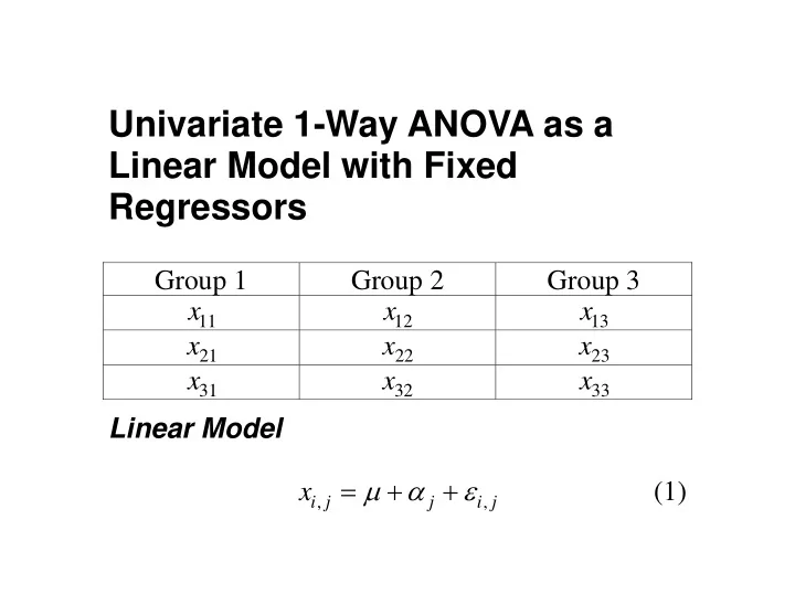
Univariate 1-Way ANOVA as a Linear Model with Fixed Regressors

Group 1 Group 2 Group 3

11

x

12

x

13

x

21

x

22

x

23

x

31

x

32

x

33

x Linear Model

, , i j j i j

x μ α ε = + + (1)

Reparameterized Linear Model

, , i j j i j

x μ ε = + (2) Matrix Form = x D ε μ + (3) D is a “design matrix” with 1’s and 0’s, and

[ ]

1 2 J

α α α μ ′ μ =

• (4)

Example.

1,1 1,1 2,1 2,1 3,1 3,1 1 1,2 1,2 2 2,2 2,2 3 3,2 3,2 1,3 1,3 2,3 2,3 3,3 3,3

1 1 1 1 1 1 1 1 1 1 1 1 1 1 1 1 1 1 x x x x x x x x x ε ε ε α ε α ε α ε μ ε ε ε ⎡ ⎤ ⎡ ⎤ ⎡ ⎤ ⎢ ⎥ ⎢ ⎢ ⎥ ⎢ ⎥ ⎢ ⎢ ⎥ ⎢ ⎥ ⎢ ⎢ ⎥ ⎡ ⎤ ⎢ ⎥ ⎢ ⎢ ⎥ ⎢ ⎥ ⎢ ⎥ ⎢ ⎢ ⎥ ⎢ ⎥ ⎢ ⎥ ⎢ = + ⎢ ⎥ ⎢ ⎥ ⎢ ⎥ ⎢ ⎢ ⎥ ⎢ ⎥ ⎢ ⎥ ⎢ ⎢ ⎥ ⎣ ⎦ ⎢ ⎥ ⎢ ⎢ ⎥ ⎢ ⎥ ⎢ ⎢ ⎥ ⎢ ⎥ ⎢ ⎢ ⎥ ⎢ ⎥ ⎢ ⎢ ⎥ ⎣ ⎦ ⎣ ⎦ ⎣ ⎥ ⎥ ⎥ ⎥ ⎥ ⎥ ⎥ ⎥ ⎥ ⎥ ⎥ ⎥ ⎦ (5)

Notice that the D matrix is not of full rank. (Why not? C.P.) D is of rank 3. We can partition D into two sub- matrices, one of which is full rank, and the other of which contains columns that are “superfluous” in the sense that they are linearly dependent.

[ ]

1 2

= D D D (6) We can similarly partition

⎡ ⎤ ⎢ ⎥ ⎣ ⎦

1 2

μ μ = μ (7) Note that we could redefine μ as

1 1 2 2 3 3

μ α μ μ α μ μ α μ + ⎡ ⎤ ⎡ ⎤ ⎢ ⎥ ⎢ ⎥ = + = ⎢ ⎥ ⎢ ⎥ + ⎢ ⎥ ⎢ ⎥ ⎣ ⎦ ⎣ ⎦

∗

μ (8) In which case

1

= + x D

∗

μ ε (9)

The null hypothesis in ANOVA can be expressed as a “general linear hypothesis” of the form ′ H

∗

μ = 0 (10) Let’s try it. Suppose 1 1 1 1 − ⎡ ⎤ ′ = ⎢ ⎥ − ⎣ ⎦ H (11) Then

1 3 1 3 2 3 2 3

α μ α μ α α α μ α μ α α + − − − ⎡ ⎤ ⎡ ⎤ ′ = = ⎢ ⎥ ⎢ ⎥ + − − − ⎣ ⎦ ⎣ ⎦ H

∗

μ (12) Notice that if both elements of the expression on the right in Equation (12) are equal, then all 3

j

α must be equal, and the null hypothesis of equal means must be true. Notice also that there are infinitely many ways you can write a “hypothesis matrix” H that expresses

the same null hypothesis. All of them will be of rank 2, or, in the case of J groups, 1 J − . Let ′ H be of order p q × , and let x have N

• elements. (Note that this N is the total N in the case
• f ANOVA.)

Under H , the following statistic has an F distribution:

( ) ( ) ( ) ( )

1 1 1 1 1 1 1 1 1 1 1 1 , 1 1 1 1 1 p N q

p F N q

− − − − − −

⎡ ⎤ ′ ′ ′ ′ ′ ′ ′ ⎢ ⎥ ⎣ ⎦ = ⎡ ⎤ ′ ′ ′ − ⎢ ⎥ ⎣ ⎦ − x D D D H H D D H H D D D x x I D D D D x

(13) This looks incomprehensible at first glance! Let’s examine the formula with reference to our simple 3 group ANOVA example, and let’s assume that sample sizes are equal in all groups. Look closely at the denominator. Note that it is the complementary projection operator for the column

space of

1

D . So the entire denominator can be written as

* *

′ ′ =

1 1

D D

x Q Q x x x . So it is a sum of squares of the projection of x into the space

• rthogonal simultaneously to all the columns of

1

D . If you study

1

D , you will see that in order for x to simultaneously be orthogonal to all the columns

• f

1

D , each group of 3 scores must have a sum of zero for its group. So this is just a fancy way of computing mean square within. Now consider the matrix expression in the

• numerator. Recognizing that

( )

1 1 1 1 −

′ ′ = D D D x x (14) On the left and the right, we have expressions of the form ′ x and x. Now, with equal n per group, it is easy to see that

1 1

n ′ = D D I (15) and so we can write the entire numerator matrix expression as

( )

1 1

n n

− −

′ ′ ′ ′ =

H

x H H IH H x x P x (16) At this point, deciphering the meaning of Equation (16) requires us to take a step back and look at

H

P . It is a column space projector for H, which has two columns in 3 dimensional space. But note that these two columns are both orthogonal to the unit vector 1, and are linearly independent. Consequently, they span the space orthogonal to 1, and so it must be that ′ = = − = − ′

H 1 1

11 P Q I P I 1 1. Consequently, the matrix quantity in Equation (16)

is simply n times the sum of squared deviations of the sample means around their overall mean. Since p in equation (13) is one less than the number of groups, we recognize that the entire expression is simply

2 2

ˆ nS F σ =

x

(17)

Two-Way ANOVA Notice that in the model

1

= x D ε

∗

μ + , all the scores in the experiment are in a single vector x, and in the hypothesis statement of Equation (10), all the means are in a single vector. Moreover, the F statistic depends on the data, N, and just two matrix quantities, i.e., the hypothesis matrix H and the design matrix

1

D . The design matrix is a simple function of the linear model in scalar form (i.e., Equation (2). However, it is less obvious how to

construct the hypothesis matrices for row, column, and interaction, effects. We need a heuristic! Constructing the Hypothesis Matrix For simplicity, suppose we have a 2 2 × ANOVA, with 2 observations per cell. The cell means are

1,1 1,2 2,1 2,2

μ μ μ μ ⎡ ⎤ = ⎢ ⎥ ⎣ ⎦ U (18)

Notice that it is easy to write the null hypothesis in the form = AUB

• 0. We can write the null

hypothesis for rows as

[ ]

1,1 1,2 2,1 2,2 1,1 1,2 2,1 2,2

1 : 1 1 1 ( ) H μ μ μ μ μ μ μ μ ⎡ ⎤ ⎡ ⎤ − ⎢ ⎥ ⎢ ⎥ ⎣ ⎦ ⎣ ⎦ = + − + = (19) This can be written

0 :

H = OU1 (20)

We call O an omnibus contrast matrix, and it is always of the same basic form, i.e.,

[ ]

= − O I 1 (21) (Examples. C.P.) In a similar vein, we can write the column effect null hypothesis as

[ ]

1,1 1,2 2,1 2,2 1,1 2,1 1,2 2,2

1 : 1 1 1 ( ) H μ μ μ μ μ μ μ μ ⎡ ⎤ ⎡ ⎤ ⎢ ⎥ ⎢ ⎥ − ⎣ ⎦ ⎣ ⎦ = + − + = (22)

This is of the form

0 :

H ′ ′ = 1 UO (23) The interaction null hypothesis is that there are no differences of differences, and consequently is of the form

0 :

H ′ = OUO (24) (C.P. Write the null hypotheses for a 3 2 × Anova row effect.)

(C.P. Write the null hypothesis for a simple main effect for columns at level 1 of the row effect.) As straightforward as this system is, unfortunately the null hypothesis requires all the means in a single vector μ, not in a matrix, and there is only

• ne hypothesis matrix, not two as in the examples
• above. So how do we proceed?

First, we need to define the Kronecker Product.

Kronecker (Direct) Product The Kronecker product of two matrices A and B is denoted ⊗ A B, and can be written in partitioned form as

1,1 1,2 1, 2,1 2,2 2, ,1 ,2 , q q p q r s p p p q

a a a a a a a a a ⎡ ⎤ ⎢ ⎥ ⎢ ⎥ ⊗ = ⎢ ⎥ ⎢ ⎥ ⎣ ⎦ B B B B B B A B B B B

• (25)

The Kronecker product above is of order pq rs × . Kronecker products have some interesting

• properties. Let vec ( )

c X be a column vector

consisting of the columns of X stacked on top of each other. Let vec ( )

r X be a column vector

consisting of the rows of X transposed into columns and stacked on top of each other. Then

( )

vec ( ) vec ( )

c c

′ = ⊗ BSA A B S (26) and, since vec ( ) vec ( )

r c

′ = S S , we also have

( )

vec ( ) vec ( )

r r

′ = ⊗ ASB A B S (27)

( )

vec ( ) vec ( )

r r

′ = ⊗ ASB A B S (28) Consider the null hypothesis of Equation (20). This can be written as

0 :

H = OU1 0, or as

( ) ( )

0 :

vecr H ′ ⊗ = O 1 U (29)

• Example. Consider the null hypothesis of no row

effect in the 2 2 × ANOVA.

( ) [ ] [ ]

( )

[ ]

1,1 1,2 2,1 2,2 1,1 1,2 2,1 2,2

1 1 1 1 1 1 1 1 μ μ μ μ μ μ μ μ ⎡ ⎤ ⎢ ⎥ ⎢ ⎥ ′ ⊗ = − ⊗ ⎢ ⎥ ⎢ ⎥ ⎣ ⎦ ⎡ ⎤ ⎢ ⎥ ⎢ ⎥ = − − ⎢ ⎥ ⎢ ⎥ ⎣ ⎦ O 1 μ

(30)

Equation (30) gives (

) ( )

1,1 1,2 2,1 2,2

μ μ μ μ + − + , which is the quantity that is zero when there is no row main effect.

General Specification of the Hypothesis Matrix in Factorial Anova

• 1. Call the effects A, B, C etc.
• 2. A conformable Omnibus Matrix for effect A is

denoted

A

O .

• 3. A conformable Summing Vector for effect A is

denoted

A

′ 1 .

• 4. A selection vector

, A j

′ s is a row vector conformable with factor A with a 1 in position j, and zeroes elsewhere.

• 1. To construct an H for a main effect, use an O

matrix for that effect and a summing vector for all

• ther effects.
• 2. To construct an H for an interaction effect, use

an O matrix for all effects in the interaction, and a summing vector for all effects not in the interaction.

• 3. To construct the H for a simple main effect, use

selection vector(s) to select the levels for the

simple main, then use an O matrix for the main effect tested.

• Examples. 2-way (

) A B × ANOVA A Main Effect

A B

′ ⊗ O 1 B Main Effect

A B

′ ⊗ 1 O AB Interaction Effect

A B

⊗ O O Simple Main Effect of A at Level 1 of B

,1 A B

′ ⊗ O s

• Examples. 3-way (

)

A B C × × ANOVA ABC Interaction Effect

A B C

⊗ ⊗ O O O A Main Effect

A B C

′ ′ ⊗ ⊗ O 1 1 Now that we understand how to express univariate ANOVA in matrix notation, we move on to MANOVA.