Overview Computational Tricks Objective Computationally efficient - - PDF document

SLIDE 1

Computational Tricks

Simon R¨ uckinger Seminar: Modeling, Simulation and Inference of Complex Biological Systems (Dr. Korbinian Strimmer) SoSe 06

• 9. Juni 2006

1 / 31

Overview

Objective Computationally efficient algorithms for quadratic regularisation Starting point A set of gene expression arrays X → large p (columns), small n (rows). Output value y we want to predict from the expression values. Idea Decompose X in a tricky way and reduce computational effort (Matrix Inversion).

2 / 31

Table of contents

1 Motivation 2 Singular value decomposition 3 Examples 4 Summary

3 / 31

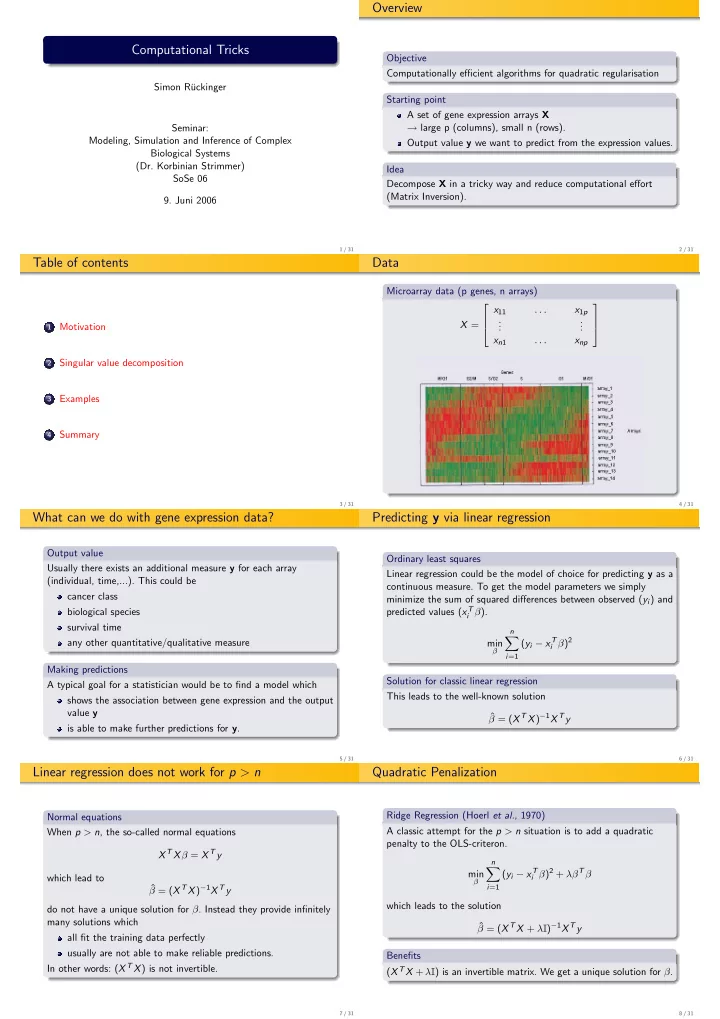
Data

Microarray data (p genes, n arrays) X =    x11 . . . x1p . . . . . . xn1 . . . xnp   

4 / 31

What can we do with gene expression data?

Output value Usually there exists an additional measure y for each array (individual, time,...). This could be cancer class biological species survival time any other quantitative/qualitative measure Making predictions A typical goal for a statistician would be to find a model which shows the association between gene expression and the output value y is able to make further predictions for y.

5 / 31

Predicting y via linear regression

Ordinary least squares Linear regression could be the model of choice for predicting y as a continuous measure. To get the model parameters we simply minimize the sum of squared differences between observed (yi) and predicted values (xT

i β).

min

β n

• i=1

(yi − xT

i β)2

Solution for classic linear regression This leads to the well-known solution ˆ β = (X TX)−1X Ty

6 / 31

Linear regression does not work for p > n

Normal equations When p > n, the so-called normal equations X TXβ = X Ty which lead to ˆ β = (X TX)−1X Ty do not have a unique solution for β. Instead they provide infinitely many solutions which all fit the training data perfectly usually are not able to make reliable predictions. In other words: (X TX) is not invertible.

7 / 31

Quadratic Penalization

Ridge Regression (Hoerl et al., 1970) A classic attempt for the p > n situation is to add a quadratic penalty to the OLS-criteron. min

β n

• i=1

(yi − xT

i β)2 + λβTβ

which leads to the solution ˆ β = (X TX + λI)−1X Ty Benefits (X TX + λI) is an invertible matrix. We get a unique solution for β.

8 / 31

SLIDE 2

Expensive Computation

Matrix Inversion (X TX + λI) is a p × p matrix. Thus the computational cost of inverting this matrix is O(p3) operations. p is large Typical expression arrays include between 1,000 and 20,000 genes. For 10,000 genes it means we have to invert a 10, 000 × 10, 000-matrix. This involves O(10, 0003) operations. How long does it take? Even on a modern PC this is a matter of hours or even days.

9 / 31

Table of contents

1 Motivation 2 Singular value decomposition 3 Examples 4 Summary

10 / 31

Getting ’tricky’

Singular value decomposition (SVD) Every Matrix X ∈ Rp×n can be decomposited in the following way X = UDV T = RV T

  X  

• nxp

=   U  

• nxn

  d1 ... dn  

• nxn

              V              

• pxn

T

11 / 31

Getting ’tricky’

Singular value decomposition (SVD) Every Matrix X ∈ Rp×n can be decomposited in the following way X = UDV T = RV T

  X  

• nxp

= R

• 

 U  

• nxn

  d1 ... dn  

• nxn

              V              

• pxn

T

11 / 31

Applying SVD to ridge regression

Another solution for ridge regression Plugging X = RV T into ˆ β = (X TX + λI)

• pxp

−1X Ty

• ne gets

ˆ β = V (RTR + λI)

• nxn

−1RTy

Conclusion We can get the parameters for ridge regression by applying SVD to X using R as a ’data-matrix’ multiplying β by V

12 / 31

About Singular Value Decomposition

Computational costs Getting the parameters for ridges regression via the SVD trick involves reducing p variables to n variables by SVD → O(pn2) solving n dimensional ridge regression → O(n3) transforming back to p dimensions → O(np) Thus it saves inverting a p × p matrix with O(p3) operations. Software SVD is a standard linear algebra tool. It is implemented in most mathematical languages. In R svd() fast.svd() → faster for small n, large p (library(corpcor))

13 / 31

Applying SVD to other models I

Linear predictors Many models ’connect’ the variables with the outcome through a linear predictor. E.g. logistic regression linear discriminant analysis support-vector machines Loss functions The parameters are estimated by minimizing a loss function n

i=1 L(yi, β0 + xT i β) which can be the

squared error negative log-likelihood etc...

14 / 31

Applying SVD to other models II

Quadratic regularization Like linear regression, all models using a linear predictor and some kind of loss function don’t work properly when p ≫ n. This can be fixed by adding a quadratic penalty min

β0,β n

• i=1

L(yi, β0 + xT

i β) + λβTβ.

The good news is The SVD trick can be used with all models in the above mentioned form. All aspects of model evaluation can be performed in this reduced space.

15 / 31

SLIDE 3

Reduced space computations

Theorem 1 Let X = RV T be the SVD of X, and denote by ri the ith row of R, a vector of n predictor values for the ith observation. Consider the pair of optimization problems: ( ˆ β0, ˆ β) = argmin

β0,β∈Rp n

• i=1

L(yi, β0 + xT

i β) + λβTβ

( ˆ θ0, ˆ θ) = argmin

θ0,θ∈Rn n

• i=1

L(yi, θ0 + rT

i θ) + λθTθ

Then ˆ β0 = ˆ θ0, and ˆ β = V ˆ θ. Proof see Hastie et al., 2004

16 / 31

Cross-validation I

Where to get λ from? The regularization parameter λ is often selected by k-fold cross-validation. How does cross-validation work? divide the training data into k groups of size n

k

fit the model to k−1

k

and test it on 1

k of the data

repeat this k seperate times average the results This is done for a series of values for λ, and a preferred value is chosen.

17 / 31

Cross-validation II

Corollary 1 The entire model-selection process via cross-validation can be performed using a single reduced data set R. Hence, when we perform cross-validation, we simply sample from the rows of R. Proof Cross-validation relies on predictions xTβ, which are equivariant under orthogonal rotations. ✷

18 / 31

Illustration / Eigengenes

X→R Eigengenes If the columns of X are centered, the columns or R are the principal components of X also called eigengenes.

19 / 31

Derivatives I

1st/2nd derivate If the loss function is based on a log-likelihood we can: perform score tests with its first derivative gain variances of the parameters from its second derivative (information matrix / hessian matrix) Expensive computation Differentation in the p-dimensional space is a waste of time. SVD once again SVD helps us to obtain the p-dimensional derivates from the n-dimensional versions.

20 / 31

Derivatives II

Corollary 2 Define L(β) =

n

• i=1

L(yi, β0 + xT

i β),

L(θ) =

n

• i=1

L(yi, β0 + rT

i θ).

Then with θ = V Tβ ⇒ L(β) = L(θ). If L is differentiable, then ∂L(β) ∂β = V ∂L(θ) ∂θ ; ∂2L(β) ∂β∂βT = V ∂2L(θ) ∂θ∂θT V T, with the partial derivatives in the right-hand side evaluated at θ = V Tβ

21 / 31

Derivatives III

Proof of Corollary 2 The euqivalence L(β) = L(θ) follows immediately from the identity X = RV T, and the fact that xT

i

and rT

i

are the ith rows of X and R. The derivatives are simple applications of the chain rule to L(β) = L(θ). ✷

22 / 31

Parenthesis: Woodbury matrix identity

Matrix inversion lemma (A + UCV )−1 = A−1 − A−1U(C −1 + VA−1U)−1VA−1 where A is p × p U is p × n C is n × n V is n × p Link to SVD For A = λI UCV = X TX = (VDUT)(UDV T) = VD2V T we see the coherency with SVD.

23 / 31

SLIDE 4

Table of contents

1 Motivation 2 Singular value decomposition 3 Examples 4 Summary

24 / 31

Where SVD can be applied

Classes of models SVD is applicable to all models in the mentioned form, of which there are many. Examples Generalized linear models The Cox proportional hazards model Multiple logistic regression Regularized linear discriminant analysis Neural networks

25 / 31

Example 1

Ramaswamy et al., 2001 Multiple logistic regression in order to predict tumor class: n = 144 training tumor samples 14 tumor classes p = 16063 genes for each sample Amount of time for parameter estimation without SVD → 8 days using SVD → 0.4 seconds

26 / 31

Example 2

My own decent example Simulation of a gene expression data set X: p = 2000 genes, n = 3 arrays (rnorm()). continuous output value y for each array (again rnorm()) Fitting a ridge regression model conventional → approx. 1 minute with SVD → less than a second see ’svd.R’ on course homepage

27 / 31

Table of contents

1 Motivation 2 Singular value decomposition 3 Examples 4 Summary

28 / 31

Summary I

Why? Estimating parameters in models for microarray data often involves inverting large (p × p) matrices. This comes along with high computational costs. How? X = RV T (SVD) R can be used as a new data matrix with dimension n × n. The p-dimensional parameter is then calculated in the following way ˆ β = V ˆ θ β ∈ Rp, θ ∈ Rn

29 / 31

Summary II

When? SVD works with all models involving a linear predictior some loss function a quadratic penalty And... Important aspects of model evaluation, such as cross-validation testing parameters can be performed with the reduced data set R. Does it afford? The time saving can be enormous!

30 / 31

Literature

Hastie, T. and Tibshirani, R. 2004. Efficient quadratic regularization for expression arrays. Biostatistics 5:329-340. Alter, O., Brown, P. and Botstein, D. 2000. Singular value decomposition for genome-wide expression data processing and modelling. Proceedings of the National Academy of Sciences, USA 97, 10101-10106 Ramaswamy, S., Tamayo, P., Rifkin, R., Mukherjee, S., Yeang, C., Angelo, M., Ladd, C., Reich, M., Latulippe, E., Mesirov, J. et al., (2001). Multiclass cancer diagnosis using tumor gene expression signature. Proceedings of the National Academy of Sciences, USA 98, 15149-15154 Hoerl, A. E., Kennard, R. W. 1970. Ridge Regression: Biased Estimation for Non-Orthogonal Problems, Technometrics, 12, 55-67.

31 / 31