Overview and Compa risons of Long-T erm Finanial Risk Mo - PDF document

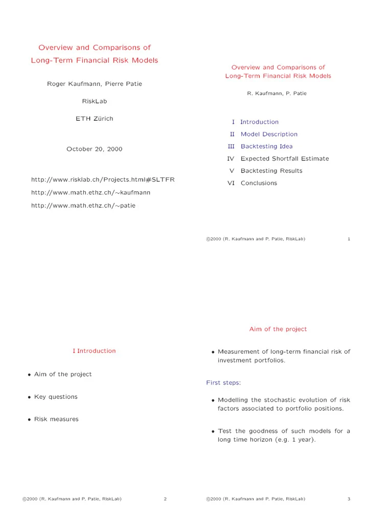
Overview and Compa risons of Long-T erm Finan ial Risk Mo dels Overview and Compa risons of Long-T erm Finan ial Risk Mo dels Roger Kaufmann, Pierre P atie R. Kaufmann, P . P atie RiskLab ETH Z� uri h I Intro du tion I I Mo del Des ription I I I Ba ktesting Idea O tob er 20, 2000 IV Exp e ted Sho rtfall Estimate V Ba ktesting Results http:/ /www.risklab. h/Proje ts.html#SL TFR VI Con lusions http:/ /www.math.ethz. h/ � k aufmann http:/ /www.math.ethz. h/ � patie � 2000 (R. Kaufmann and P . P atie, RiskLab) 1 Aim of the p roje t I Intro du tion � Measurement of long-term �nan ial risk of investment p o rtfolios. � Aim of the p roje t First steps: � Key questions � Mo delling the sto hasti evolution of risk fa to rs asso iated to p o rtfolio p ositions. � Risk measures � T est the go o dness of su h mo dels fo r a long time ho rizon (e.g. 1 y ea r). � 2000 (R. Kaufmann and P . P atie, RiskLab) 2 � 2000 (R. Kaufmann and P . P atie, RiskLab) 3

Risk measure de�nition 60 W e onsider as risk measure the exp e ted sho rt- fall. 40 De�nition 1 The exp e ted sho rtfall ES at a � 20 level � is de�ned b y 1 ( R ) = � E [ R j R � V ( R )℄ ; 2 (�) : ES < aR where R L � � yearly returns in % 0 2 ℄0 ; 1[ , De�nition 2 Given � the value-at-risk VaR(5%) V aR at level � of the returns R with distribu- � tion P , is -20 � f x 2 j � � � g ; V aR ( R ) = inf R P [ R x ℄ � ES(5%) i.e. V aR is the negative of the � -quantile of R . -40 The exp e ted sho rtfall is a risk mea- oherent -60 sure in the sense of Artzner, Delbaen, Eb er and Heath. In general, value-at-risk is not ! P&L distribution � 2000 (R. Kaufmann and P . P atie, RiskLab) 4 � 2000 (R. Kaufmann and P . P atie, RiskLab) 5 Key questions 1. Whi h frequen y do w e use to �t mo dels? � Are long datasets stationa ry? � What a re the statisti al restri tions? I I Mo del Des ription (la k of y ea rly returns) � Ho w an w e k eep as mu h info rmation � Random W alk as p ossible? � GARCH(1,1) 2. Do the p rop erties of �nan ial data hange when w e ho ose another time ho rizon? � Heavy-tailed distribution 3. What is the reliabilit y of the time aggrega- tion rule of ea h mo del if there is any? 4. Ho w an w e ompa re di�erent time ho ri- zons and mo dels? � 2000 (R. Kaufmann and P . P atie, RiskLab) 6 � 2000 (R. Kaufmann and P . P atie, RiskLab) 7

GARCH(1,1) Random W alk Let ( X ; t 2 N ) b e a stri tly stationa ry time t Assumption 1: exp e ted log returns a re equal series rep resenting observations of entered log to zero returns on a �nan ial asset p ri e. [ r ℄ = 0 : E t t +1 Assumption 2: No rmally distributed, inde- A GARCH(1,1) mo del fo r is de�ned b y X p endent log returns with standa rd deviation � = fo r 2 in ea h p erio d [ t; t + 1℄. X � � t N ; t t t 2 2 2 = + + � � � X � � ; 0 1 t � 1 1 t � 1 t iid 2 Ass. 1 & 2 ) s N (0 ; ) : r � 2 t +1 � iid ; E [ � ℄ = 0 ; E [ � ℄ = 1 : t t t ! The loga rithmi asset p ri e follo ws a ran- Stationa rit y onditions: dom w alk with zero drift. 0 1 , � 0, � 0 and + 1 : < � < � � � � < 0 1 1 1 1 Time aggregation: h � 1 X Fit the GARCH(1,1) p ro ess b y pseudo-maximum- iid 2 r := r s N (0 ; h� ) : t � i h;t lik eliho o d estimation to obtain the value of the i =0 pa rameters of the onditional volatilit y . � 2000 (R. Kaufmann and P . P atie, RiskLab) 8 � 2000 (R. Kaufmann and P . P atie, RiskLab) 9 Time aggregation: GARCH o eÆ ients fun - Heavy-tailed distributions tion W e onsider ( r ; t 2 N ) to b e indep endent and Assume: Centered 1-da y log returns follo w X t t identi ally distributed (i.i.d.), rep resenting ob- a GARCH(1,1) p ro ess with a no rmally dis- servations of the log returns on a �nan ial as- tributed innovation. set p ri e. = X � � ; t t t W e assume 2 2 2 = + + � � � X � � ; 0 1 t � 1 1 t � 1 t � � P [ r < � x ℄ = C x L ( x ) as x ! 1 ; (1) iid 1 � s N (0 ; 1) : t + where C ; � 2 R and L is a slo wly va rying fun tion, i.e. Drost-Nijman: L ( tx ) h � 1 8 t 0 : lim = 1 : X > x !1 L ( x ) X : = X is w eak GARCH(1,1): t � i h;t i =0 X = � � ; Distributions satisfying (1) a re alled heavy- h;t h;t h;t sin e the th moment is tailed distributions k 2 2 2 � = � + � X + � � ; h; 0 h; 1 h; 1 h;t h;t � 1 h;t � 1 in�nite fo r � . (1) is also a ha ra terisation k > iid N (0 ; 1) ; � s h;t of the maximum domain of attra tion of the F r e het � distribution. ! 0 ; ! 0 as ! 1 : � � h h; 1 h; 1 � 2000 (R. Kaufmann and P . P atie, RiskLab) 10 � 2000 (R. Kaufmann and P . P atie, RiskLab) 11

Time aggregation F eller's theo rem (1971) ( r 2 N ) Theo rem: Assuming that ; t have heavy- t tailed distributions leads to 2 3 h X � � 4 5 � x = L ( x ) x [1 + o (1)℄ ; ! 1 ; P r < hC fo r x t t =1 where the s ale fa to r C is as in (1) . I I I Ba ktesting Idea P h o rresp onds to the h -da y log returns. r t t =1 � Mo del ompa rison When appli able, this theo rem supplements the entral limit theo rem b y p roviding info rmation on erning the tails. � Ba ktesting des ription Da o rogna, M� uller, Pi tet and de V ries sho w the follo wing theo rem: Supp ose has a �nite va rian e (i.e. 2). r � > A t a onstant risk level p , in reasing the time ho rizon h in reases the V aR and the exp e ted sho rtfall numb ers fo r the heavy tailed mo del 1 b y a fa to r . h � � 2000 (R. Kaufmann and P . P atie, RiskLab) 12 � 2000 (R. Kaufmann and P . P atie, RiskLab) 13 Ba ktesting: T est Des ription Idea: ompa re fo re asted exp e ted sho rtfall Mo del Compa rison d ES with empiri al estimation of exp e ted t;� sho rtfall. No one of the p rop osed mo dels obviously out- p erfo rms the others. Ea h of them has its Measure 1: Evaluate values b elo w the negative de� ien ies. d of the estimated value-at-risk V aR . t;� All mo dels only p erfo rm w ell fo r relatively sho rt W e build the di�eren e b et w een the real (i.e. ob- time ho rizons. W e have to �x a ho rizon h < served) one-y ea r returns and the negative R 1 y ea r, fo r whi h w e an use our mo dels. F o r t +1 d of the estimation ES . the gap b et w een h and 1 y ea r, w e will have to t;� W e al ulate the onditional average of these use a s aling rule. d di�eren es, onditioned on f R � g , < V aR t +1 t;� � � P t d 1 � ( � ES ) 1 R t +1 t;� d t = t 0 f R < � V aR g ES t;� t +1 V = : P 1 scaling rule t 1 1 suitable model t = t d f R < � V aR g 0 t +1 t;� today h 1 year A go o d estimation fo r exp e ted sho rtfall will ES lead to a lo w absolute value of V . 1 � 2000 (R. Kaufmann and P . P atie, RiskLab) 14 � 2000 (R. Kaufmann and P . P atie, RiskLab) 15