[PPT] - Outline Overview of Game Theory A. Introduction Models of PowerPoint Presentation

SLIDE 1

Outline

A. Introduction
B. Single Agent Learning
C. Game Theory
D. Multiagent Learning
E. Future Issues and Open Problems

SA3 – C1

Overview of Game Theory

Models of Interaction

– Normal-Form Games – Repeated Games – Stochastic Games

Solution Concepts

SA3 – C2

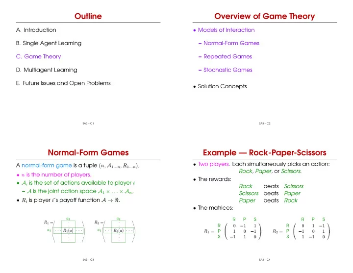
Normal-Form Games

A normal-form game is a tuple

✁ ✂☎✄ ✆✞✝✠✟ ✟ ✟ ✡ ✄ ☛ ✝ ✟ ✟ ✟ ✡ ☞

,

✂

is the number of players,

✆✍✌

is the set of actions available to player

✎

–

✆

is the joint action space

✆ ✝ ✏✒✑ ✑ ✑ ✏ ✆ ✡

,

☛✓✌

is player

✎

’s payoff function

✆ ✔ ✕

.

. . . . . . . . . . . . . . . . . . . . . .

✖ ✗ ✖ ✘ ✖ ✘ ✖ ✗ ✙ ✘ ✚ ✙ ✗ ✛ ✖ ✜ ✙ ✘ ✛ ✖ ✜ ✙ ✗ ✚

SA3 – C3

Example — Rock-Paper-Scissors

Two players. Each simultaneously picks an action:

Rock, Paper, or Scissors.

The rewards:

Rock beats Scissors Scissors beats Paper Paper beats Rock

The matrices:

✢✤✣ ✥

R P S

✦ ✧ ★

R

✩ ✪

P

✪

S

✪ ★ ✩ ✪ ✩ ✪ ✪ ★ ✫ ✬ ✢✤✭ ✥

R P S

✦ ✧ ★

R

✪

P

✩ ✪

S

✩ ✪ ★ ✪ ✪ ✩ ✪ ★ ✫ ✬

SA3 – C4

SLIDE 2

More Examples

Matching Pennies

✢ ✣ ✥

H T

✪

H

✩ ✪

T

✩ ✪ ✪ ✁ ✢ ✭ ✥

H T

✩

✪

H

✪

T

✪ ✩ ✪ ✁

Coordination Game

✢ ✣ ✥

A B

✂

A

★

B

★ ✪ ✁ ✢ ✭ ✥

A B

✂

A

★

B

★ ✪ ✁

Bach or Stravinsky

✢ ✣ ✥

B S

✂

B

★

S

★ ✪ ✁ ✢✤✭ ✥

B S

✪

B

★

S

★ ✂ ✁

SA3 – C5

More Examples

Prisoner’s Dilemma

✢✤✣ ✥

C D

✄

C

★

D

☎ ✪ ✁ ✢✤✭ ✥

C D

✄

C

☎

D

★ ✪ ✁

Three-Player Matching Pennies

SA3 – C6

Three-Player Matching Pennies

Three players. Each simultaneously picks an action:

Heads or Tails.

The rewards:

Player One wins by matching Player Two, Player Two wins by matching Player Three, Player Three wins by not matching Player One.

SA3 – C7

Three-Player Matching Pennies

The matrices:

✢✤✣ ✆✝ ✞ ✟ ✞ ✟ ✠ ✡☛ ✥

H T

✪

H

★

T

★ ✪ ✁ ✢✤✣ ✆ ✝ ✞ ✟ ✞ ✟ ☞ ✡☛ ✥

H T

✪

H

★

T

★ ✪ ✁ ✢ ✭ ✆✝ ✞ ✟ ✞ ✟ ✠ ✡☛ ✥

H T

✪

★ ✪ ★ ✁ ✢ ✭ ✆ ✝ ✞ ✟ ✞ ✟ ☞ ✡☛ ✥

H T

★

✪ ★ ✪ ✁ ✢✍✌ ✆✝ ✞ ✟ ✞ ✟ ✠ ✡☛ ✥

H T

★

★ ✪ ✪ ✁ ✢✍✌ ✆ ✝ ✞ ✟ ✞ ✟ ☞ ✡☛ ✥

H T

✪

✪ ★ ★ ✁

SA3 – C8

SLIDE 3

Strategies

What can players do?

– Pure strategies (

✌

): select an action. – Mixed strategies (

✁ ✌

): select an action according to some probability distribution.

SA3 – C9

Strategies

Notation.

–

✁

is a joint strategy for all players.

☛✓✌ ✁ ✁ ☞ ✂ ✄ ☎ ✆ ✝ ✁ ✁

☞

☛✓✌ ✁

☞

–

✁✟✞ ✌

is a joint strategy for all players except

✎

. –

✠ ✁ ✌ ✄ ✁✟✞ ✌ ✡

is the joint strategy where

✎

uses strategy

✁ ✌

and everyone else

✁ ✞ ✌

.

SA3 – C10

Types of Games

Zero-Sum Games (a.k.a. constant-sum games)

☛ ✝ ☛ ☛✌☞ ✂ ✍

Examples: Rock-paper-scissors, matching pennies.

Team Games

✎ ✎ ✄ ✏ ☛ ✌ ✂ ☛✒✑

Examples: Coordination game.

General-Sum Games (a.k.a. all games)

Examples: Bach or Stravinsky, three-player matching pennies, prisoner’s dilemma

SA3 – C11

Repeated Games

You can’t learn if you only play a game once.
Repeatedly playing a game raises new questions.

– How many times? Is this common knowledge? Finite Horizon Infinite Horizon – Trading off present and future reward?

✓ ✔✖✕ ✗ ✘ ✙ ✝ ✗ ✚ ✗✜✛ ✢ ✝ ✣ ✛ ✚ ✙ ✛ ✢ ✝ ✤ ✛ ✣ ✛

Average Reward Discounted Reward

SA3 – C12

SLIDE 4

Repeated Games — Strategies

What can players do?

– Strategies can depend on the history of play.

✁ ✌

✁

✔ ✂✄ ✁ ✆ ✌ ☞

where

✁ ✂ ✙ ☎ ✡ ✢ ✆ ✆ ✡

– Markov strategies a.k.a. stationary strategies

✎

✝✠✟

✟ ✟ ✡ ✝ ✆ ✁ ✌ ✁

✝

✄ ✑ ✑ ✑ ✄

✡

☞ ✂ ✁ ✁

✡

☞

–

✞

Markov strategies

✎

✝

✟ ✟ ✟ ✡ ✝ ✆ ✁ ✌ ✁

✝

✄ ✑ ✑ ✑ ✄

✡

☞ ✂ ✁ ✁

✡

✞ ✟ ✄ ✑ ✑ ✑ ✄

✡

☞

SA3 – C13

Repeated Games — Examples

Iterated Prisoner’s Dilemma

✢✤✣ ✥

C D

✄

C

★

D

☎ ✪ ✁ ✢✤✭ ✥

C D

✄

C

☎

D

★ ✪ ✁

– The single most examined repeated game! – Repeated play can justify behavior that is not rational in the one-shot game. – Tit-for-Tat (TFT)

✠

Play opponent’s last action (C on round 1).

✠

A 1-Markov strategy.

SA3 – C14

Stochastic Games

Multiple State
Multiple Agent
Single State
Multiple Agent

Repeated Games

Multiple State

MDPs

Single Agent

SA3 – C15

Stochastic Games — Definition

A stochastic game is a tuple

✁ ✂ ✄ ✡ ✄ ✆ ✝ ✟ ✟ ✟ ✡ ✄ ☛ ✄ ☛ ✝ ✟ ✟ ✟ ✡ ☞

,

✂

is the number of agents,

✡

is the set of states,

✆

✌

is the set of actions available to agent

✎

, –

✆

is the joint action space

✆ ✝ ✏✒✑ ✑ ✑ ✏ ✆ ✡

,

☛

is the transition function

✡ ✏ ✆ ✏ ✡ ✔ ☞ ✍ ✄ ✌ ✍

,

☛✓✌

is the reward function for the

✎

th agent

✡ ✏ ✆ ✔ ✕

.

. . . . . . . . . . .

✎ ✏ ✑ ✒✔✓✖✕ ✎ ✕ ✓ ✗✘ ✓ ✓ ✗ ✙ ✏ ✒ ✓✖✕ ✎ ✘ ✎ ✚ ✙ ✏ ✒ ✓ ✘✜✛

SA3 – C16

SLIDE 5

Stochastic Games — Policies

What can players do?

– Policies depend on history and the current state.

✌
✁

✏ ✡ ✔ ✂✄ ✁ ✆ ✌ ☞

where

✁ ✂ ✙ ☎ ✡ ✢ ✆ ✁ ✡ ✏ ✆ ☞ ✡

– Markov polices a.k.a. stationary policies

✎✁ ✄ ✁ ✂ ✝ ✁ ✎☎✄ ✝ ✡

✌

✁ ✁ ✄ ✄ ☞ ✂

✁

✁ ✂ ✄ ✄ ☞

– Focus

n

learning Markov policies, but the learning itself is a non-Markovian policy.

SA3 – C17

Example — Soccer

(Littman, 1994)

A B

Players: Two.
States: Player positions and ball possession (780).
Actions: N, S, E, W, Hold (5).
Transitions:

– Simultaneous action selection, random execution. – Collision could change ball possession.

Rewards: Ball enters a goal.

SA3 – C18

Example — Goofspiel

Players hands and the deck have cards

✌ ✑ ✑ ✑ ✂

.

Card from the deck is bid on secretly.
Highest card played gets points equal to the card

from the deck.

Both players discard the cards bid.
Repeat for all

✂

deck cards.

✆ ✝ ✞ ✝ ✝ ✞ ✟ ✠ ✝

SIZEOF(

✡

r

☛

) V(det) V(random) 4 692 15150

☞

59KB

✩ ✂ ✩ ✂✍✌ ✎

8

✄ ✟ ✪ ★ ✏ ✪ ✟ ✪ ★ ✑ ☞

47MB

✩ ✂ ★ ✩ ✪ ★✍✌ ✎

13

✪ ✟ ✪ ★ ✣ ✣ ✒ ✟ ✪ ★ ✣ ✣ ☞

2.5TB

✩ ✓ ✎ ✩ ✂✔

SA3 – C19

Stochastic Games — Facts

If

✂ ✂ ✌

, it is an MDP .

If

✕ ✖ ✕ ✂ ✌

, it is a repeated game.

If the other players play a stationary policy, it is an

MDP to the remaining player.

✗ ☛ ✁ ✄ ✄

✌

✄ ✄ ✂ ☞ ✂ ✄ ☎✙✘ ✚ ✆ ✝ ✘ ✚ ✟✞ ✌ ✁ ✄ ✄

☞

☛ ✁ ✄ ✄ ✠

✌

✄

✞

✌ ✡ ✄ ✄ ✂ ☞

– The interesting case, then, is when the other agents are not stationary, i.e., are learning.

SA3 – C20

SLIDE 6

Overview of Game Theory

Models of Interaction
Solution Concepts

Normal Form Games – Dominance – Minimax – Pareto Efficiency – Nash Equilibria – Correlated Equilibria Repeated/Stochastic Games – Nash Equilibria – Universally Consistent

SA3 – C21

Dominance

An action is strictly dominated if another action is

always better, i.e,

✂

✌ ✝ ✆✍✌ ✎

✞

✌ ✝ ✆ ✞ ✌ ☛✓✌ ✁ ✠

✂

✌ ✄

✞

✌ ✡ ☞ ✁ ☛✓✌ ✁ ✠

✌

✄

✞

✌ ✡ ☞ ✑

Consider prisoner’s dilemma.

✢✤✣ ✥

C D

✄

C

★

D

☎ ✪ ✁ ✢✤✭ ✥

C D

✄

C

☎

D

★ ✪ ✁

– For both players, D dominates C.

SA3 – C22

Iterated Dominance

Actions may be dominated by mixed strategies.

Consider matching pennies.

✢ ✣ ✥

H T

✪

H

✩ ✪

T

✩ ✪ ✪ ✁ ✢✤✭ ✥

H T

✩

✪

H

✪

T

✪ ✩ ✪ ✁

Q: What do we do when the world is out to get us?

A: Make sure it can’t.

Play strategy with the best worst-case outcome.

✂ ✄ ☎ ✕ ✂ ✆ ✝ ✚ ✆ ✞ ✟ ✝ ✚ ✠ ✕ ✔ ✡ ☎ ✘ ✚ ✆ ✝ ✘ ✚ ☛✓✌ ✁ ✠ ✁ ✌ ✄ ✁ ✞ ✌ ✡ ☞

Minimax optimal strategy.

SA3 – C24

SLIDE 7

Minimax

Back to matching pennies.

✢ ✣ ✥

H T

✪

H

✩ ✪

T

✩ ✪ ✪ ✁

✪
✂

✪

✂

✁ ✥ ✁ ✂ ✣

Consider Bach or Stravinsky.

✢✤✣ ✥

B S

✂

B

★

S

★ ✪ ✁

✪
✄

✂

✄

✁ ✥ ✁ ✂ ✣

Minimax optimal guarantees the saftey value.
Minimax optimal never plays dominated strategies.

SA3 – C25

Minimax — Linear Programming

Minimax optimal strategies via linear programming.

✂ ✄ ☎ ✕ ✂ ✆ ✝ ✚ ✆ ✞ ✟ ✝ ✚ ✠ ✕ ✔ ✡ ☎✙✘ ✚ ✆ ✝ ✘ ✚ ☛✓✌ ✁ ✠ ✁ ✌ ✄ ✁ ✞ ✌ ✡ ☞ ✄ ☎ ✆ ✝

SA3 – C26

Pareto Efficiency

A joint strategy is Pareto efficient if no joint strategy is

better for all players, i.e.,

✎

✂

✝ ✆

✎

✝ ✌ ✄ ✑ ✑ ✑ ✄ ✂ ☛✓✌ ✁

☞

✞ ☛✓✌ ✁

✂

☞

In zero-sum games, all strategies are Pareto efficient.

SA3 – C27

Pareto Efficiency

Consider prisoner’s dilemma.

✢✤✣ ✥

C D

✄

C

★

D

☎ ✪ ✁ ✢✤✭ ✥

C D

✄

C

☎

D

★ ✪ ✁

–

✠ ✄ ✄ ✄ ✡

is not Pareto efficient.

Consider Bach or Stravinsky.

✢ ✣ ✥

B S

✂

B

★

S

★ ✪ ✁ ✢✤✭ ✥

B S

✪

B

★

S

★ ✂ ✁

–

✠ ✟ ✄ ✟ ✡

and

✠ ✖ ✄ ✖ ✡

are Pareto efficient.

SA3 – C28

SLIDE 8

Nash Equilibria

What

action should we play if there are no dominated actions?

Optimal action depends on actions of other players.
A best response set is the set of all strategies that are
ptimal given the strategies of the other players.
✁

✌ ✁ ✁✟✞ ✌ ☞ ✂ ✂ ✁ ✌ ✕ ✎ ✁ ✂ ✌ ☛ ✌ ✁ ✠ ✁ ✌ ✄ ✁✟✞ ✌ ✡ ☞ ✞ ☛ ✌ ✁ ✠ ✁ ✂ ✌ ✄ ✁✟✞ ✌ ✡ ☞✄

A Nash equilibrium is a joint strategy, where all

players are playing best responses to each other.

✎ ✎ ✝ ✂ ✌ ✑ ✑ ✑ ✂ ✄ ✁ ✌ ✝

✁

✌ ✁ ✁✟✞ ✌ ☞

SA3 – C29

Nash Equilibria

A Nash equilibrium is a joint strategy, where all

players are playing best responses to each other.

✎ ✎ ✝ ✂ ✌ ✑ ✑ ✑ ✂ ✄ ✁ ✌ ✝

✁

✌ ✁ ✁ ✞ ✌ ☞

Since each player is playing a best response, no

player can gain by unilaterally deviating.

Dominance solvable games have obvious equilibria.

– Strictly dominated actions are never best responses. – Prisoner’s dilemma has a single Nash equilibrium.

SA3 – C30

Examples of Nash Equilibria

Consider the coordination game.

✢✤✣ ✥

A B

✂

A

★

B

★ ✪ ✁ ✢ ✭ ✥

A B

✂

A

★

B

★ ✪ ✁

Consider Bach or Stravinsky.

✢✤✣ ✥

B S

✂

B

★

S

★ ✪ ✁ ✢ ✭ ✥

B S

✪

B

★

S

★ ✂ ✁

SA3 – C31

Examples of Nash Equilibria

Consider matching pennies.

✢ ✣ ✥

H T

✪

H

✩ ✪

T

✩ ✪ ✪ ✁ ✢ ✭ ✥

H T

✩

✪

H

✪

T

✪ ✩ ✪ ✁

– No pure strategy Nash equilibria. Mixed strategies?

✁

✝ ☎ ✠ ✌ ✆ ✝ ✄ ✌ ✆ ✝ ✡ ✞ ✂ ✂ ✁ ✝ ✄

– Corresponds to the minimax strategy.

SA3 – C32

SLIDE 9

Existence of Nash Equilibria

All finite normal-form games have at least one Nash
equilibrium. (Nash, 1950)
In zero-sum games. . .

– Equilibria all have the same value and are interchangeable.

✠ ✁ ✝ ✄ ✁ ☞ ✡ ✄ ✠ ✁ ✂ ✝ ✄ ✁ ✂ ☞ ✡

are Nash

✠

✁ ✝ ✄ ✁ ✂ ☞ ✡

is Nash

✑

– Equilibria correspond to minimax optimal strategies.

SA3 – C33

Computing Nash Equilibria

The

exact complexity

f

computing a Nash equilibrium is an open problem. (Papadimitriou, 2001)

Likely to be NP-hard. (Conitzer & Sandholm, 2003)
Lemke-Howson Algorithm.
For two-player games, bilinear programming solution.

SA3 – C34

Fictitious Play

(Brown, 1949; Robinson 1951)

An iterative procedure for computing an equilibrium.
1. Initialize

✁ ✌ ✁

✌

✝ ✆✍✌ ☞

, which counts the number of times player

✎

chooses action

✌

.

2. Repeat.

(a) Choose

✌

✝ ✟ ☛ ✁ ✁ ✞ ✌ ☞

. (b) Increment

✁ ✌ ✁

✌

☞

.

SA3 – C35

Fictitious Play

(Fudenberg & Levine, 1998)

If

✁ ✌

converges, then what it converges to is a Nash equilibrium.

When does

✁ ✌

converge? – Two-player, two-action games. – Dominance solvable games. – Zero-sum games.

This could be turned into a learning rule.

SA3 – C36

SLIDE 10

Correlated Equilibria

Is there a way to be fair in Bach or Stravinsky?

✢ ✣ ✥

B S

✂

B

★

S

★ ✪ ✁ ✢ ✭ ✥

B S

✪

B

★

S

★ ✂ ✁

– Suppose we wanted to both go to Bach or both go to Stravinsky with equal probability? – We want to correlate our action selection.

B S

✪
✂

B

★

S

★ ✪

✂

✁

but not B S

✪
☎

B

✪

☎

S

✪

☎

✪

☎

✁

SA3 – C37

Correlated Equilibria

Assume a shared randmoizer (e.g., a coin flip) exists.
Define a new concept of equilibrium.

– Let

✁

be a probability distribution over joint actions. – Each player observes their own action in a joint action sampled from

✁

. –

✁

is a correlated equilibrium if no player can gain by deviating from their prescribed action.

✎ ✎

✌

✝

✁

✌ ✁ ✁ ✞ ✌ ✕ ✁ ✄

✌

☞

SA3 – C38

Correlated Equilibria

Back to Bach or Stravinsky.

✢ ✣ ✥

B S

✂

B

★

S

★ ✪ ✁ ✢ ✭ ✥

B S

✪

B

★

S

★ ✂ ✁ ✁ ✥

B S

✪
✂

B

★

S

★ ✪

✂

✁

All Nash equilibria are correlated equilibria.
All mixtures of Nash are correlated equilibria.

SA3 – C39

Overview of Game Theory

Models of Interaction
Solution Concepts

Normal Form Games – Dominance – Minimax – Pareto Efficiency – Nash Equilibria – Correlated Equilibria Repeated/Stochastic Games – Nash Equilibria – Universally Consistent

SA3 – C40

SLIDE 11

Nash Equilibria in Repeated Games

Obviously, Markov strategy equilibria exist.
Consider iterated prisoner’s dilemma and TFT.

✢✤✣ ✥

C D

✄

C

★

D

☎ ✪ ✁ ✢✤✭ ✥

C D

✄

C

☎

D

★ ✪ ✁

– With average reward, what’s a best response?

✠

Always D has a value of 1.

✠

D then C has a value of 2.5

✠

Always C and TFT have a value of 3. – Hence, both players following TFT is Nash.

SA3 – C41

Nash Equilibria in Repeated Games

The TFT equilibria is strictly preferred to all Markov

strategy equilibria.

The TFT strategy plays a dominated action.
TFT uses a threat to enforce compliance.
TFT is not a special case.

SA3 – C42

Nash Equilibria in Repeated Games

Folk Theorem. For any repeated game with average reward, every feasible and enforceable vector of payoffs for the players can be achieved by some Nash equilibrium strategy. (Osborne & Rubinstein, 1994)

A payoff vector is feasible if it is a linear combination
f individual action payoffs.
A payoff vector is enforceable if all players get at

least their minimax value.

SA3 – C43

Nash Equilibria in Repeated Games

Folk Theorem. For any repeated game with average reward, every feasible and enforceable vector of payoffs for the players can be achieved by some Nash equilibrium strategy. (Osborne & Rubinstein, 1994)

Players’ follow a deterministic sequence of play that

achieves the payoff vector.

Any deviation is punished.
The threat keeps players from deviating as in TFT.

SA3 – C44

SLIDE 12

Computing Repeated Game Equilibria

(Littman & Stone, 2003)

Polynomial

time algorithm for finding a Nash equilibrium in a repeated game. – Find a feasible and enforceable payoff vector. – Construct a strategy that punishes deviance.

SA3 – C45

Universally Consistent

A.k.a. Hannan consistent, regret minimizing.
For a history

✁ ✂

✝

✄

☞

✄ ✑ ✑ ✑ ✄

✡

✝ ✆

, define regret for player

✎

, Regret

✌ ✁ ✁ ☞ ✂

✕

✂ ✆ ☎ ✚ ✆ ✝ ✚ ✡ ✄ ✛ ✢ ✝ ☛ ✁ ✁

✌

✄

✛

✞ ✌ ✂ ☞ ✄ ☎ ✡ ✄ ✛ ✢ ✝ ☛✓✌ ✁

✛

☞

i.e., the difference between the reward that could have been received by a stationary strategy and the actual reward received.

SA3 – C46

Universally Consistent

A strategy

✁ ✌

is universally consistent if for any

✆ ✁ ✍

there exists a

☛

such that for all

✁ ✞ ✌

and

✝ ✁ ☛

,

✞ ✄ ✟

Regret

✌ ✠

✝

✄ ✑ ✑ ✑ ✄

✛

✡ ✝ ✁ ✆ ☛☞☛✌☛✍☛ ✠ ✁ ✌ ✄ ✁ ✞ ✌ ✡ ✎ ✏ ✆

i.e., with high probability the average regret is low for all strategies of the other players.

If regret is zero, then must be getting at least the

minimax value.

SA3 – C47

Nash Equilibria in Stochastic Games

Consider Markov policies.
A best response set is the set of all Markov policies

that are optimal given the other players’ policies.

✁✓✌

✁

✞

✌ ☞ ✂ ✑

✌

✕ ✎

✂

✌ ✎ ✄ ✝ ✡ ✒ ✠✔✓ ✚ ✕ ✓ ✘ ✚ ✡ ✌ ✁ ✄ ☞ ✞ ✒ ✠ ✓ ✖ ✚ ✕ ✓ ✘ ✚ ✡ ✌ ✁ ✄ ☞ ✗

A Nash equilibrium is a joint policy, where all players

are playing best responses to each other.

✎ ✎ ✝ ✂ ✌ ✑ ✑ ✑ ✂ ✄

✌

✝

✁

✌ ✁ ✟✞ ✌ ☞

SA3 – C48

SLIDE 13

Nash Equilibria in Stochastic Games

All

discounted reward and zero-sum average reward stochastic games have at least one Nash

equilibrium. (Shapley, 1953; Fink, 1964)
Stochastic games are the general model.
Nash equilibria in stochastic games has certainly

received the most attention.

SA3 – C49